
Take any finite network of one-way arrows, forbid loops and opposing arrows, and look two steps ahead. Must somebody reach at least as many new vertices in two steps as in one? The Seymour second neighborhood conjecture says yes. OpenAI’s September 23, 2026 paper proves this for every nonempty finite oriented graph. Its argument assumes that a graph where every vertex fails exists, amplifies that assumption into strict inequalities for vertex subsets, then forces a counting objective beyond its maximum. Understanding why that hypothetical graph cannot exist requires distinguishing new destinations from repeated paths.
Table of Contents
1. What Is Seymour’s Second Neighborhood Conjecture?
An oriented graph assigns directions to the edges of a simple undirected graph. It need not be complete or connected. Write for an arc, and for the vertices reached directly from . The second out-neighborhood, , contains vertices reached in two steps after excluding and all direct out-neighbors.
A vertex satisfying this inequality is a Seymour vertex. The paper’s Theorem 1.1 guarantees at least one. A sink, meaning a vertex without outgoing arcs, qualifies because both counts vanish.
| Item | Verified Statement |
|---|---|
| Paper | A proof of Seymour’s second-neighborhood conjecture, OpenAI, September 23, 2026. |
| Setting | Nonempty finite oriented graphs. Loops, multiple arcs, and opposite arc pairs are excluded. |
| Conclusion | At least one vertex has as many exact second out-neighbors as first out-neighbors. |
| Core Mechanism | Subset deficit, transitive-tournament blowup, and an extremal contradiction using pruning. |
| Scope | No connectivity or degree assumption. A sink qualifies. No runtime benchmark is supplied. |
The second neighborhood problem concerns distinct destinations, not numbers of walks. Removing direct neighbors makes the assertion substantially stronger than merely comparing all one-step and two-step endpoints.
2. A Simple Directed Graph That Reveals the Two-Step Puzzle
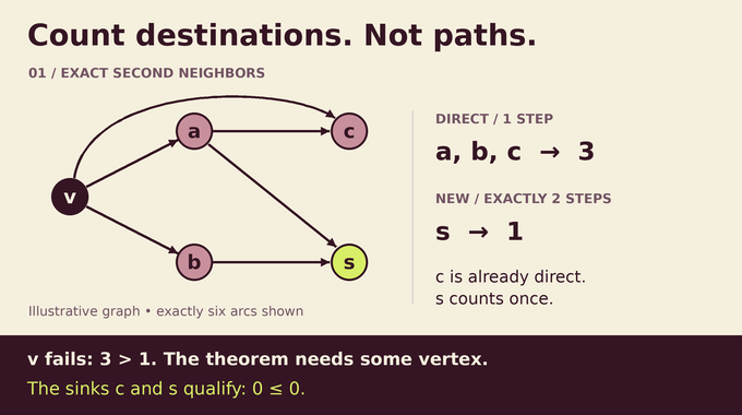
For a concrete example of the Seymour second neighborhood conjecture, take five vertices . Include exactly these arcs: , , , , , and .
From , two-step walks reach once and twice. However, is already a direct neighbor, while duplicate arrivals at count only once. Thus the first count is three and the exact second count is one.
| Vertex | First Out-Neighbors | Exact Second Out-Neighbors | Qualifies? |
|---|---|---|---|
| No: | |||
| No: | |||
| No: | |||
| Yes: | |||
| Yes: |
The failure at does not refute the theorem. The quantifier is “some vertex,” and both sinks work. This example also explains why simply squaring an adjacency matrix is insufficient: its entries count walks, whereas the theorem requires distinct endpoints with direct neighbors removed.
3. Why Earlier Proofs Could Not Settle the General Case
A tournament has exactly one arc between every pair of distinct vertices. Fisher proved the tournament case, and Havet and Thomassé supplied a combinatorial proof using local median orders. Missing edges destroy that complete interaction pattern, so tournament arguments do not automatically cover arbitrary orientations.
The paper also records proofs for minimum outdegree at most six and a computer-assisted preprint addressing seven. Minimum outdegree means the smallest outgoing degree anywhere in the graph. These results leave graphs whose minimum exceeds those thresholds untreated.
Earlier universal ratio bounds guarantee a vertex with a second neighborhood at least a fixed fraction of its first. The introduction cites approximately 0.657298, later 0.715538, and a reported computational bound of 0.74530. Every constant remains below the required one. These are mathematical guarantees, not benchmark scores. As with other graph conjectures involving structural restrictions, proving special cases requires careful attention to which hypotheses remain.
4. The Proof Begins with a Minimal Counterexample
Assume every vertex in some oriented graph has fewer exact second out-neighbors than first out-neighbors. Choose such a graph with the fewest vertices, then the fewest arcs among graphs of that order. These two minimality conditions serve different purposes.
First, has no sink. Second, it is strongly connected: every vertex can reach every other along directed paths. Otherwise, choose a strongly connected component with no outgoing arc to another component. All first and second out-neighborhoods of its vertices stay inside it, producing a smaller counterexample.
Strong connectivity and the absence of sinks ensure more than one vertex and positive indegree everywhere. Later, minimality of the arc count will ensure that deleting certain arcs creates a qualifying vertex. No original connectivity assumption has been added to the theorem. Connectivity is deduced only for the hypothetical smallest obstruction.
5. How Arc Deletion Creates the Crucial Subset Inequality
Define as all vertices receiving an arc from some member of , and let . Unlike an exact second neighborhood, this ordinary image operator does not subtract previously visited vertices.
Fix a nonempty proper subset . Put and . Strong connectivity makes nonempty. Grow an auxiliary subset from empty to , tracking .
At each stage, delete all arcs from to , starting afresh from the original graph. Arc minimality supplies a vertex that now qualifies. It must have lost an outgoing neighbor, so it lies in . Let be its nonempty set of lost neighbors.
The set identifies second neighbors lost after deletion. Comparing gains and losses yields . Summing these strict increments proves Lemma 2.2:
Subtracting on the right is the crucial strengthening. A weaker bound by all of would not supply the later amplification.
The loss comparison must also account for vertices that become newly eligible for the exact second neighborhood. Deleting an arc creates no new path, but it can remove a direct connection to a vertex still reachable in two steps. Such a vertex was previously excluded. The proof explicitly charges those gains against lost direct neighbors, preventing a misleading monotonicity argument about exact second neighborhoods.
6. Why the Proof Replaces Vertices with Transitive Tournaments,
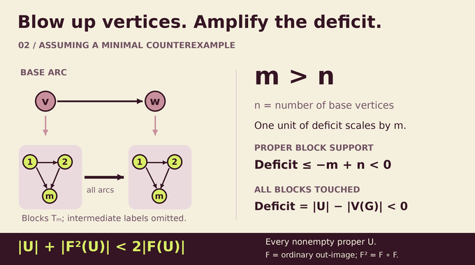
Replace every vertex of by a transitive tournament with vertices, where and is the order of . Within each block, labels point from smaller to larger. Each original arc becomes every possible arc between the corresponding blocks, directed consistently.
This blowup is the lexicographic product . One unit of integer deficit in the base graph now contributes an entire block of size . Internal block effects cost at most , giving a bound at most when the selected blocks form a proper subset of base vertices.
If a proper subset of blowup vertices touches every block, positive indegrees instead make its first and second ordinary images the whole graph. This separate case is essential. Together, the estimates give Proposition 2.1: a hypothetical counterexample produces a graph satisfying
The construction amplifies a contradiction hypothesis. It is not a model of measured network growth.
7. From Vertex Sets to Two Families of Ordered Pairs
Set . Work with two families . The operator advances the first coordinate along an arc and fixes the second. The operator advances the second coordinate and fixes the first.
Call the families compatible when . Both must contain the diagonal . Taking both families equal to that diagonal is initially compatible, since an overlap would require opposite arcs.
Let and . Compatibility makes the number of uncovered ordered pairs. Among all allowed pairs of families, maximize .
Every column of and row of is nonempty because it contains its diagonal entry. Each is proper because positive indegrees and compatibility exclude full columns and rows. Consequently, the strict subset inequality applies separately to every column and row. This transfers a statement about vertices into controlled counting across a square grid.
Why include uncovered points in the objective at all? Maximizing only the combined family size would leave the eventual deletions uncompensated. Adding their number builds the anticipated correction into the quantity being optimized. Finiteness ensures this is a genuine attained maximum, rather than a limiting value that larger families might approach indefinitely.
8. The Pruning Lemma: Removing Conflicts Without Losing Too Much
Lemma 3.1 considers arbitrary finite binary relations, not only oriented graphs. A left member conflicts with a right member when and .
Each conflict determines two points. Put in and in . A left member covers a point by advancing its first coordinate, while a right member covers one by advancing its second coordinate. A conflict therefore means both sides cover the same point of .
Pruning retains subfamilies with no conflicts, preserves every initially conflict-free member, and bounds deletions by . Here counts points of uncovered after pruning.
That final qualification drives the proof. Removing members can create uncovered points, so charging against the original uncovered set alone would be inadequate. The extremal objective deliberately rewards uncovered points, allowing their increase to compensate for the corresponding deletion cost. The two families remain separate copies even when their coordinates agree.
The preservation clause is equally important. The final application requires diagonal members to survive, so merely finding some compatible subfamilies would not suffice. Initially conflict-free members are isolated in the augmented graph, and the chosen cover omits isolated vertices. This supplies exactly the retention guarantee the extremal construction needs.
9. How Bipartite Matchings and Matrix Ranks Make Pruning Work
Construct an augmented bipartite graph with original members and two separate copies of . Edges represent conflicts or coverage. A vertex cover meets every edge. Kőnig’s theorem equates minimum vertex-cover size with maximum matching size, connecting the argument to maximum-cardinality matching.
The required bound is a matching size at most . Four linear maps encode changes of coordinates. Two routes from a left member to a right member pass through different index sets, but their entries agree:
Here maps from the space indexed by to that indexed by , and maps onward to the space indexed by . The alternative route uses through , followed by .
Coefficients are chosen simultaneously so relevant supported matrices attain maximum rank. The kernel lemma says a right-kernel coordinate and a left-kernel coordinate cannot both be nonzero at an allowed entry of a maximum-rank supported matrix. Otherwise, perturbing that entry would increase rank.
Combined with independent kernel vectors and rank–nullity, this bounds the matching. The reasoning concerns rank and support, distinct from counting perfect matchings, although determinant expansions connect both subjects. Our permanent versus determinant explainer provides related matrix background.
To obtain the deletion bound from a cover, delete only original family members lying in that cover. Every conflict disappears. For each previously conflicting point still covered by a survivor, an opposite copy of that point must itself belong to the cover. These compulsory copies consume part of the cover budget. Subtracting their count leaves precisely the allowance involving the conflict set and the points subsequently uncovered.
10. The Final Contradiction: Why the Counterexample Cannot Survive
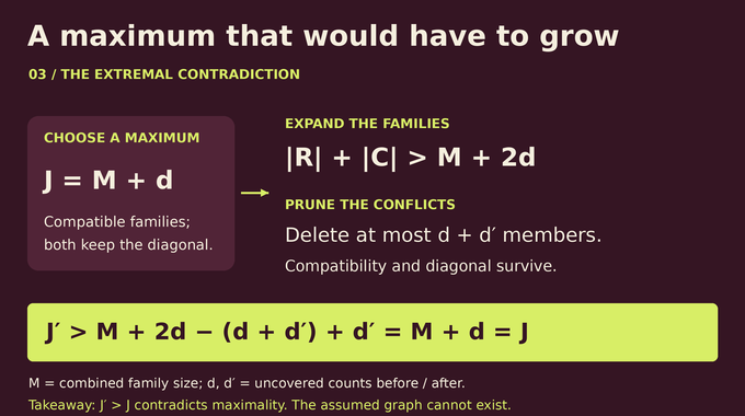
Return to the maximizing compatible families. Take complements of their iterated coordinate images: and . Summing the strict subset inequalities gives .
Both new families contain the diagonal, and every diagonal member is conflict-free. A forbidden conflict involving such a member would create a two-step coordinate path placing its partner inside the image whose complement defined the family.
Apply pruning. Every point of was previously uncovered, so . Let count all points uncovered by the retained families. At most points of remain uncovered, making the deletion cost at most .
The retained families are compatible and still contain the diagonal, yet their objective exceeds its chosen maximum. Proposition 4.1 therefore excludes the graph that Proposition 2.1 would produce. This closes the Seymour second neighborhood conjecture proof.
11. What Else Follows from the Proof?
Through Seacrest’s established equivalences, the result yields weighted versions. For every nonnegative vertex weighting, some vertex has second-neighborhood weight at least first-neighborhood weight. Separately, there exists a nonnegative weighting of total mass one making that comparison hold at every vertex. These quantifier orders differ, and zero weights are allowed. The paper also states the corresponding arc-weighted form.
Directed-cycle consequences follow because, without directed triangles, exact second out-neighbors are neither incoming nor outgoing neighbors. For some vertex, this yields , where the superscripts denote outgoing and incoming degrees.
Hence minimum indegree and minimum outdegree both at least force a directed triangle. Both conditions matter. The result does not assert the same conclusion from minimum outdegree alone. If every incoming and outgoing degree equals and directed girth is exactly four, then . Girth means shortest directed-cycle length. These consequences follow directly from the neighborhood comparison.
For the triangle conclusion, absence of a triangle would force the sum of twice the minimum outdegree and the minimum indegree to be at most the order minus one. The two stated degree thresholds make that sum at least the order, an immediate contradiction including the endpoint case.
12. What the OpenAI Proof Establishes and Its Precise Scope
OpenAI’s Seymour conjecture proof concerns nonempty finite oriented graphs, including disconnected graphs and sinks. It does not directly cover arbitrary digraphs or infinite graphs. Without orientation, two vertices joined by opposite arcs already violate the proposed inequality at both vertices.
The Lean scope note identifies the main existence theorem as formalized. Its comparator configuration points to a separate solution module, whose proof invokes reduction, pruning, and the extremal contradiction. The comparator statement’s placeholder is therefore distinct from the solution. This article does not report an independent compilation or extend the documented scope to every corollary. See our Lean proof explainer and AI mathematical proofs guide for related reading.
For an explicitly given graph, checking every vertex’s first and exact second neighborhoods is polynomial-time work. The achievement is universal existence, not a new search benchmark. The Seymour second neighborhood conjecture becomes a theorem because every hypothetical obstruction forces an impossible strict increase. Follow Binary Verse AI for research explainers that connect precise statements to the arguments establishing them.
What is a Seymour vertex in graph theory?
A Seymour vertex is a vertex satisfying . It has at least as many distinct vertices at directed distance exactly two as it has immediate out-neighbors.
Does the second neighborhood include vertices already reachable in one step?
No. The second out-neighborhood counts vertices whose shortest directed distance is exactly two. The starting vertex and vertices reachable directly are excluded, even if a two-step walk also reaches them.
Why does the proof use a transitive-tournament blowup?
Replacing each vertex with a sufficiently large transitive tournament amplifies a strict subset deficit. With block size , where is the base graph’s order, it produces the stronger inequality for every nonempty proper subset needed by the later extremal argument.
What is the role of the pruning lemma in OpenAI’s proof?
The pruning lemma removes conflicting members from two families of ordered pairs while controlling how many are deleted. Its bound involves both original conflict data and points left uncovered afterward, allowing the final contradiction.
Can a Seymour vertex actually be found algorithmically?
Yes. For a finite, explicitly given oriented graph, an algorithm can inspect each vertex’s first and exact second out-neighborhoods and find a qualifying vertex in polynomial time. The paper’s main contribution is proving that such a vertex always exists, not introducing that basic search procedure.
Does the proof apply to every directed graph, including infinite graphs?
The stated theorem applies to nonempty finite oriented graphs, which exclude loops, multiple arcs, and pairs of opposite arcs. It does not directly assert the same theorem for arbitrary directed graphs or infinite graphs.