
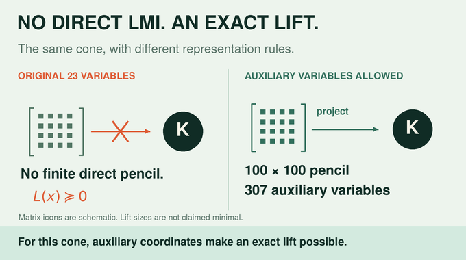
A convex cone can pass every real-root test in its definition and still resist every finite matrix description in its original coordinates. OpenAI’s September 24, 2026 manuscript gives an explicit example: a hyperbolicity cone in 23 real variables, ultimately defined by a degree-16 polynomial, that is not spectrahedral. This disproves the geometric generalized Lax conjecture. The result excludes all finite direct symmetric linear matrix inequalities, rather than merely one proposed determinant formula. It does not exclude auxiliary variables: a separate October paper constructs an exact semidefinite lift of this very cone.
Table of Contents
01. What Did OpenAI Prove About the Generalized Lax Conjecture?
Theorem 1.1 of A Nonspectrahedral Hyperbolicity Cone establishes the obstruction using a degree-20 polynomial. Corollary 1.2 removes a redundant factor and obtains degree 16. Both polynomials define the same closed cone.
| Feature | Verified Statement |
|---|---|
| Coordinates | Two symmetric 4 × 4 matrices and one three-dimensional vector: 23 real variables. |
| Degree | 20 initially; 16 after removing a determinant factor. |
| Excluded | Every finite direct homogeneous real symmetric matrix pencil. |
| Separate Result | The same closed cone has an exact semidefinite lift. |
This is a mathematical existence theorem with an explicit construction, not a solver benchmark. The supplied PDF presents an ordinary written proof. OpenAI’s release announcement discusses Lean formalizations of many results, but that release-wide statement does not establish formal verification of this particular theorem. Our guide to OpenAI’s mathematical proofs provides broader context.
02. The Original Problem: Hyperbolic Polynomials, Convex Cones and Matrices
A homogeneous polynomial has all monomials of the same total degree. It is hyperbolic with respect to a vector when and every root of is real for every real . Its closed hyperbolicity cone consists of inputs for which those roots are nonnegative, including zero. Gårding’s theory guarantees convexity.
Write for real symmetric matrices. Positive semidefiniteness, , means that every quadratic form value is nonnegative. A spectrahedral cone has a direct linear matrix inequality:
For example, the symmetric matrix with rows and is positive semidefinite exactly when , , and . These three scalar conditions describe one cone through a two-by-two matrix. The conjecture predicted an analogous finite matrix description for every hyperbolicity cone, however large the required matrix.
For a numerical check, choose both diagonal entries equal to one and the off-diagonal entry equal to one-half. The determinant is three-quarters and the eigenvalues are one-half and three-halves, both positive. Increasing the off-diagonal entry beyond one makes the determinant negative. This elementary example shows how a linear matrix inequality encodes a nonlinear boundary.
03. Why Earlier Counterexamples Could Not Settle the Geometric Conjecture
The original three-variable Lax problem has a positive answer through the Helton–Vinnikov determinantal representation theorem. Higher dimensions require separating two questions: can this polynomial be a definite determinant, and can this cone be defined by some matrix pencil?
Brändén’s determinantal obstruction ruled out representations for every positive power of a particular real-zero polynomial. Nevertheless, another determinant with additional factors might define the same cone. Kummer’s specialized Vámos example makes that distinction concrete: its cone has a seven-by-seven representation despite the obstruction for powers of its defining polynomial.
This is different from the polynomial-complexity questions in our permanent versus determinant explainer. Here the object being ruled out is every finite pencil defining a fixed set. Positive results under stronger hypotheses also survive. The paper’s example is not strictly hyperbolic: along a specified nonradial line, its root polynomial has repeated factors.
A definite determinantal representation requires a symmetric matrix pencil that is positive definite at the hyperbolicity direction and whose determinant equals the chosen polynomial. Cone equality demands less algebraic agreement: extra factors are allowed if their signs do not impose new restrictions. That additional freedom is precisely what earlier polynomial obstructions left unresolved.
04. Building OpenAI’s Explicit 23-Variable Counterexample
Take and . Each symmetric four-by-four matrix contributes ten independent entries, giving . With cyclic indices modulo three, define the Choi–Lam biquadratic form:
The symmetric matrix satisfies , with diagonal entries and off-diagonal entries . For a scalar , vector , and , set
This map is linear in its matrix input and quadratic in . The adjugate, , is the transpose of the cofactor matrix, satisfying . Now define
Write for its closed hyperbolicity cone in direction . Every entry inside the determinant has degree five: either four from the determinant and one from , or three from the adjugate and two from . The four-by-four determinant therefore has degree 20. Crucially, the adjugate formula remains polynomial at singular .
The distinction between polynomiality and linearity matters. A compact determinant expression is not automatically a spectrahedral description. Its entries must be linear in the original coordinates, and a determinant inequality alone does not establish positive semidefiniteness. The construction deliberately combines polynomial matrix entries with a separate root-based definition of its cone.
- Choi–Lam form: scalar nonnegativity with a rigid obstruction.
- Positive map: encode that form in symmetric matrices.
- Determinant polynomial: obtain a hyperbolicity cone in 23 variables.
05. The Choi–Lam Lemma: A Nonnegative Form That Dominates No Bilinear Square
Lemma 2.1 contains the obstruction. First write and view the form as a quadratic expression in . Its matrix has diagonal . Its off-diagonal entries are the negative pairwise products of the coordinates of . For each cyclic index, its two-by-two principal minor is . Its determinant is
The arithmetic–geometric mean inequality proves this last inequality. Consequently all principal minors are nonnegative, proving . Yet , so the form is not zero.
For the determinant inequality, the three positive terms have product equal to the cube of the subtracted product. Their sum is therefore at least three times that product. Nonnegative diagonal entries and the remaining principal minors complete the positive-semidefiniteness test. Testing only the determinant would not have been sufficient for a symmetric three-by-three matrix.
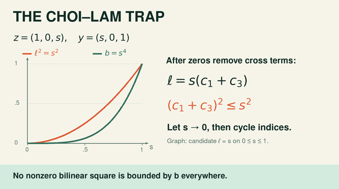
Suppose a bilinear form satisfies everywhere. At zeros of , it must vanish. The coordinate zeros remove three coefficients. Evaluating at the eight sign vectors and averaging against gives . Together these identities remove every off-diagonal coefficient.
For the remaining diagonal coefficients, take the cyclic index , so and . Direct substitution gives
The bound forces for nonzero . Letting and cycling indices makes all three diagonal coefficients zero. Thus no nonzero bilinear square lies beneath this nonnegative form.
06. Why the Constructed Polynomial Is Actually Hyperbolic
Nonnegativity first makes the matrix map positive. Split vectors in as and . Direct multiplication yields
Every positive semidefinite matrix is a nonnegative sum of rank-one matrices, so preserves positive semidefiniteness. For invertible , the determinant formula becomes
To exclude nonreal roots, put with . The inverse has negative definite imaginary part. Positivity of the complex-linearly extended map makes the imaginary part of at least , hence positive definite. That matrix cannot be singular. Neither determinant factor vanishes in the upper half-plane.
Real coefficients exclude lower-half-plane roots by conjugation. At , the polynomial equals one, so its directional polynomial always has degree 20. All its roots are real. This establishes hyperbolicity independently of the later argument against matrix representations.
The imaginary-part argument uses complex matrices only to locate roots of a real polynomial. It does not replace the positive map by a claim of complete positivity. Ordinary preservation of positive semidefiniteness on real symmetric inputs supplies exactly the order comparison needed for the inverse matrix’s imaginary part.
07. Two Cone Slices That Reveal the Matrix Structure
Proposition 3.2 identifies the positive-definite slice and the zero-vector slice exactly:
For the first equivalence, consider . If , order preservation gives for positive . If its least eigenvalue starts negative, it eventually becomes positive and must cross zero. The resulting determinant zero is incompatible with cone membership.
The second slice follows directly from eigenvalues of and , including zero eigenvalues. It also explains why arbitrary negative matrix directions cannot be hidden inside a representing pencil. The strict first-slice inequalities give an open neighborhood of inside the cone. These are exact membership statements, not numerical tests.
The restriction to positive definite first matrices is deliberate because their inverses exist. It is not a complete inverse-based formula for singular boundary points. The polynomial definition supplies those points without division, and the zero-vector slice includes them explicitly. Keeping these two descriptions separate prevents an unjustified extension of the Schur-complement condition. Their convex-geometric setting connects with our Mahler conjecture explainer.
08. Assuming a Matrix Representation: Compression, Rescaling and Schur Complements
Proposition 4.1 assumes an arbitrary finite pencil. Since is interior, the kernel of its value there is common to the whole pencil and can be removed. The zero-vector slice then isolates two nonzero blocks. Congruence normalizes their positive maps so that each sends identity to identity.
Rescale inputs as . The quadratic dependence of preserves the slice condition. Positivity for both signs of eliminates the lower diagonal term linear in . A block congruence and the limit leave diagonal blocks and off-diagonal block , linear in .
The converse requires care: perturb to . Because , this makes the limiting block matrix positive definite. Nearby rescaled matrices are then feasible. Letting recovers the original inequality. The output dimensions of these maps are fixed by the assumed pencil. They may be arbitrarily large, but they remain finite throughout the proof. Positivity and normalization ensure that a positive definite input gives a positive definite first block, so its inverse and the Schur complement are legitimate. The Schur complement gives
09. Rank-One Limits Produce the Exact Operator-Norm Identity
For unit vectors , set and , with . Their inverses suppress directions perpendicular to the chosen vectors. Meanwhile, and converge to the kernel projections
Substituting into the preceding equivalence identifies two closed rays of admissible real thresholds . Their endpoints are respectively a largest eigenvalue and a squared operator norm. Equality of those endpoints survives the rank-one limit:
The operator norm measures maximum Euclidean stretching, the matrix language also encountered in our Crouzeix inequality explainer. Here exact equality is essential. A mere upper estimate would not reconstruct the Choi–Lam form. At , the left side is zero, forcing the entire matrix product to vanish.
To see the projection limit, diagonalize a fixed positive semidefinite matrix. In the inverse square root of identity plus a growing multiple of that matrix, a zero eigenvalue contributes one. Every positive eigenvalue contributes a factor tending to zero. Thus the limit retains exactly the kernel, including cases where that kernel is trivial.
10. The Tangent-Space Contradiction That Completes OpenAI’s Proof
Choose with where the rank of is maximal on that part of the unit sphere. Nearby independent columns persist, giving constant rank and a smooth kernel projection . Keep fixed.
For , move along . Define . Subtract the zero matrix product at , divide by , and pass to the limit:
Only is differentiated. The map is injective because would make parallel to . Both spaces have dimension three, so it is an isomorphism. Substituting produces a matrix bilinear in .
Every entry’s square is bounded by the squared operator norm, which equals . Lemma 2.1 makes every entry vanish. The equality would then force itself to vanish, contradicting . No finite pencil can survive this contradiction.
Although the differentiation takes place locally on a sphere, the resulting bound covers every pair of three-dimensional vectors. The tangent-space isomorphism supplies all first inputs, while the second input was arbitrary from the beginning. This explains why a local calculation can invoke the globally quantified Choi–Lam lemma and exclude a representation of the whole cone.
11. From Degree 20 to Degree 16: The Final Counterexample and Its Limits
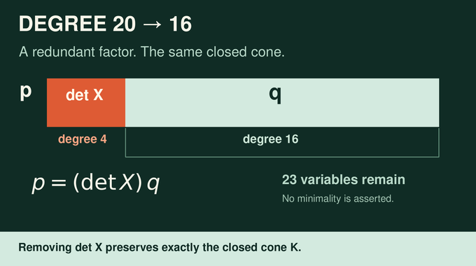
Section 7 constructs a larger block determinant proving the polynomial identity . This establishes divisibility even at singular matrices. The quotient has degree 16 and inherits real-rootedness from . Removing a factor could enlarge a cone, so equality still needs proof.
Because is even in , convexity puts in its cone whenever belongs. At zero , , forcing . The removed determinant therefore imposed no additional cone restriction.
| Question | Answer |
|---|---|
| Direct finite matrix representation? | Impossible for this cone. |
| Smallest possible counterexample? | No dimension or degree minimality is asserted. |
| Representation with auxiliary variables? | Possible for this cone by the separate October construction. |
The October 5 exact-lift paper gives a size-100 pencil with 307 auxiliary variables for the entire closed cone. These sizes are not claimed minimal. Neither paper supplies practical solver-performance measurements.
A semidefinite representation with a lift asks whether there exists a choice of auxiliary coordinates making the enlarged pencil positive semidefinite. Projecting its feasible set recovers the original cone. Those existential coordinates are exactly the freedom forbidden in the direct representation problem. The October result therefore complements the September obstruction without reversing it.
The real symmetric convention also closes a possible loophole involving complex Hermitian pencils. A Hermitian matrix can be converted into a real symmetric block matrix with equivalent positivity, so such a direct pencil would contradict the same theorem. The counterexample establishes an unrestricted impossibility in matrix size, rather than a lower bound that a sufficiently large direct matrix might eventually overcome. The generalized Lax conjecture fails because convex real-root geometry exceeds direct matrix expressibility. Auxiliary coordinates change that answer. As in our Kohn–Sham representability explainer, identifying the permitted representation is essential. Follow Binary Verse AI for source-led explanations that keep the theorem, mechanism, and limitations together.
Is the generalized Lax conjecture true or false?
The geometric generalized Lax conjecture is false in full generality. OpenAI’s September 24, 2026 manuscript proves that an explicit hyperbolicity cone cannot be represented by any finite direct homogeneous real symmetric linear matrix inequality. The original three-variable Lax theorem remains valid.
What is a nonspectrahedral hyperbolicity cone?
It is the closed convex cone associated with a hyperbolic polynomial that has no direct description by any finite real symmetric linear matrix pencil. OpenAI constructs an explicit example in 23 real variables.
Why did earlier counterexamples not disprove the geometric conjecture?
Earlier obstructions excluded definite determinant representations of particular polynomials or their positive powers. They did not exclude a different determinant, potentially with extra factors, defining the same cone. This argument excludes every finite direct representing pencil for its cone.
Why is the Choi–Lam biquadratic form essential to the proof?
The form is nonnegative and nonzero, but no nonzero bilinear form has its square bounded above by it everywhere. The proof converts a hypothetical pencil into a bilinear matrix whose entries satisfy exactly that bound. Every entry must vanish, contradicting the nonzero form.
How does OpenAI prove its polynomial is hyperbolic?
The Choi–Lam form gives a positive linear map. For each real input, the determinant formula and a positive imaginary-part argument exclude roots in the upper half-plane. Real coefficients exclude their conjugates in the lower half-plane. Thus every directional root is real.
Why does the paper mention both degree 20 and degree 16?
The initial construction produces a degree-20 polynomial in 23 variables. Section 7 proves that it contains the factor . Removing this factor gives a degree-16 hyperbolic polynomial. A separate cone argument verifies that the removal does not change the closed cone.
Does the counterexample mean the cone cannot have a semidefinite lift?
No. The September paper excludes direct matrix representations in the original variables. The separate October 5 paper constructs an exact semidefinite lift of this same closed cone, including singular boundary points, using a size-100 pencil and 307 auxiliary variables. No minimality of these sizes is asserted.