
A quadratic wave can oscillate furiously while three shifted copies conceal its cancellation. That is the central difficulty behind the trilinear Hilbert transform. OpenAI’s October 5, 2026 manuscript proves the fixed-slope estimate for slopes 1, 2, 3. Its contribution is a method for controlling matched quadratic structure across arbitrarily many scales. The result settles this exponent case, rather than the entire conjecture. Below, we follow the argument from its symmetry to the final uniform bound, while separating the manuscript’s theorem from later extensions and reported proof issues.
Table of Contents
01. What OpenAI’s L³ Proof Actually Establishes
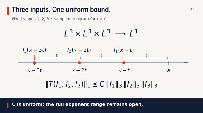
Theorem 1.1 of OpenAI’s original manuscript, An L³ Bound for the Trilinear Hilbert Transform, states that a finite constant controls the output norm by the product of three input norms:
Initially, the inputs are Schwartz functions, meaning smooth functions whose derivatives decay rapidly. Density then gives a unique bounded trilinear extension to all three input spaces. The constant is independent of the inputs. This is the precise L3 bound for the trilinear Hilbert transform developed in the paper.
| Question | Verified Scope |
|---|---|
| Operator | Straight-line shifts with slopes 1, 2, 3 |
| Input and output | Three inputs, one output |
| Uniformity | No growth with the number of scales |
| What remains | The full conjectured exponent range |
| Evidence | October 5 manuscript, with later review issues discussed below |
02. The Original Trilinear Hilbert Transform Problem
The operator multiplies three translated functions and integrates against the singular kernel :
Principal value means removing a symmetric interval around zero before taking its width to zero. The symmetry preserves cancellation between positive and negative displacements. For Schwartz inputs, decay handles the distant tails. Absolute integration near zero would discard the cancellation on which the operator depends.
Here is the real line. Membership in means that the integral of the absolute cube is finite, with norm . An output has finite integral of its absolute value. The exponent relation matches the proposed mapping.
The trilinear Hilbert transform conjecture asks for stable bounds for whole classes of inputs. Computing one integral, or observing convergence for smooth examples, cannot establish that stability. Related questions about operator estimates appear in our Crouzeix conjecture explainer, although its operators and geometry differ.
There is a useful stability consequence: small changes to any one input, measured in its input norm, produce controlled changes in the output when the other two inputs have bounded norms. This follows from trilinearity and the displayed estimate. It explains why extending from smooth functions is mathematically substantive, rather than a change of notation.
03. Why Previous Hilbert Transform Methods Were Not Enough
Lacey and Thiele established the bilinear predecessor, involving two shifted inputs. Adding a third introduces quadratic modulation symmetry in the associated four-linear form. The challenge is therefore structural, rather than simply a longer version of the bilinear calculation.
Terence Tao’s work on cancellation for the multilinear Hilbert transform improved an elementary logarithmic truncation bound to a sublogarithmic one. That was genuine cancellation, but a quantity growing more slowly can still grow without limit. OpenAI needs a bound that stays finite as the truncation spans more scales.
Curved variants supply another important distinction. Their nonlinear shifts create oscillation through curvature. The introduction cites Hu and Lie’s results but explains that these do not settle the straight-line operator here. Changing the shifts changes the mechanism available to the proof.
For neighboring harmonic-analysis context, our local smoothing and Kakeya conjecture explainers examine different ways oscillation and geometry shape estimates. Their conclusions are not ingredients of this argument.
04. The Quadratic Phase Identity at the Heart of the Difficulty
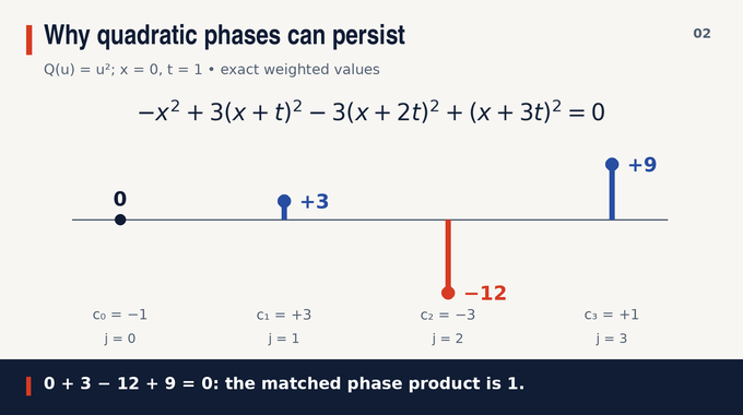
Pairing the output with a bounded test function introduces a fourth input, . After reversing the integration variable, the progression coordinates become x, x+t, x+2t, x+3t. Reversal changes the operator’s sign, not its norm. The coefficients below annihilate every polynomial through degree two:
| Moment | Explicit Weighted Sum | Total |
|---|---|---|
| Constant | −1 + 3 − 3 + 1 | 0 |
| Linear | 0 + 3 − 6 + 3 | 0 |
| Quadratic | 0 + 3 − 12 + 9 | 0 |
For a worked example, expand the squares:
The coefficients of the squared spatial variable, the mixed product, and the squared displacement each vanish. With , multiplying the four corresponding quadratic phase factors therefore gives exactly one. Envelopes can remain, but this source of oscillatory cancellation disappears.
This explains why rapidly varying inputs need not be harmless. The proof must recognize their shared structure. Our Littlewood polynomial explainer offers another setting where organized phases matter, without implying the same theorem.
For another check, take the quadratic polynomial to be the square function and choose spatial position zero with displacement one. The four weighted values are zero, three, minus twelve, and nine. Their sum vanishes exactly. The signed chart displays this arithmetic, rather than suggesting that the entire singular integral must vanish.
05. From Local Singular Integrals to a Scale-Independent Estimate
Section 2 replaces the global kernel with smooth local four-linear forms attached to dyadic intervals. Dyadic refinement halves interval length at each depth. Each kernel is supported where all four progression coordinates remain inside its interval, and has cancellation along each of the four anchor directions.
For collections occupying at most consecutive depths, the paper defines through an absolute local-form sum bounded by an integral of four maximal functions. These maximal functions measure nearby averages of the inputs. Their auxiliary exponent satisfies . A straightforward estimate grows linearly with .
The target is an absorption inequality, schematically after fixed constants are incorporated:
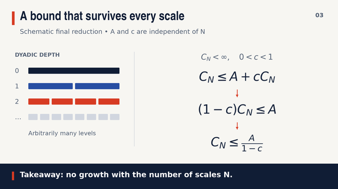
The unknown constant is already finite on a finite tree. Thus a sufficiently small coefficient lets the argument move its own contribution to the left. The work is proving that small coefficient without allowing the supposedly fixed remainder to depend on depth.
06. Detecting Quadratic Structure with Higher-Order Uniformity
Section 4 begins with quantitative Weyl alternatives for quadratic charts. Roughly, an appreciable oscillatory average forces arithmetic structure in its parameters. Otherwise cancellation makes that average small. The quantitative bounds matter because this detection will be used repeatedly.
The external structural input is the degree-two case of the Leng–Sah–Sawhney inverse theorem for Gowers uniformity norms. A bounded function with substantial norm correlates with a controlled degree-two nilsequence. Such structured sequences generalize simple quadratic exponentials. Replacing them all by one ordinary quadratic would misdescribe the proof.
The manuscript builds continuous quadratic charts and localization statements from that discrete input. Its bounded-input decomposition separates structured approximations from a remainder small in the relevant uniformity sense. Local progression forms then detect structure when the remainder still contributes appreciably.
This is a detector, not a complete summation theorem. Detecting structure on one interval leaves open how the resulting descriptions interact along a long chain of descendants. The next construction addresses precisely that bookkeeping cost.
A quadratic chart packages oscillation together with smooth cutoffs and auxiliary periodic coordinates. Ordinary quadratic exponentials are included as a special case. The larger class remains manageable under conjugation, multiplication, and affine rescaling, which the local argument repeatedly needs. Its complexity bounds are part of the quantitative estimate, rather than decorative descriptions of structure.
07. Private Coordinates and Compression Across Arbitrarily Many Scales
Section 3 augments each scalar column with a private orthogonal direction:
The scalar component enters the singular integral. The extra direction records that particular label. Even identical scalar columns receive different private directions, making their coefficients recoverable. Positive private weights prevent coefficient recovery from becoming arbitrarily ill-conditioned within the stated budget.
Projection masks inherit columns on descendants. Lemma 3.4 controls products of these local projections acting before rows with a joint square-energy bound. For a fixed number of factors, the cost is a power of the logarithm of the budget , rather than a power of spatial depth.
That budget includes column sizes, inverse private-coordinate sizes, and labels born along a single spatial path. Labels on disjoint branches can be arbitrarily numerous. This distinction prevents a large global catalog from becoming a false depth restriction. Compression preserves the quantitative room needed for later errors to remain small.
The square-energy hypothesis has a concrete purpose. Orthogonal increments can be accumulated through the sum of their squared norms, instead of adding their magnitudes one by one. Compression lets the argument insert the required inherited projections while retaining that advantage. It does not say that arbitrary products of arbitrary projections have logarithmic cost.
08. Two Accuracies, Delayed Projections, and the Base Reduction
Section 5 constructs approximations at staggered accuracies. A later fit is chosen substantially more accurate than earlier fits, so its errors can dominate the costs already incurred. Predictor moments monitor interactions when two structured arguments are fixed.
The delayed projections are evaluated on finer partitions while decisions are assigned to coarser cells. Rolling differences measure changes between projections. Orthogonal energy bounds make their squared sizes summable, avoiding an absolute charge at every intervening depth.
The resulting base reduction has small pair interactions and a controlled active collection. On each normalized segment, only a budgeted number of scales remain active along a path. This count may depend on accuracy, but not on the original total depth.
Stopping a summation does not erase auxiliary functions already used on ancestor cells. Their inherited projections continue by refitting below the stop. Exceptional summands restart on smaller roots whose lengths have a geometric packing bound. That consistency is essential when later estimates refer back to earlier projections.
09. Localizing Quadratic Curvature and Controlling Side Terms
Section 6 assigns normalized curvature tags to the original columns and groups compatible tags through a graph. Linear modulation is excluded from the tag. The grouping therefore tracks quadratic compatibility without confusing it with ordinary frequency shifts.
Historical masks preserve separation when projection adjoints act on earlier cells. Transferring complementary filters then creates coupled narrow-band defects. These cannot simply be declared negligible or split into independently summable pieces.
Section 7 handles them on short depth blocks. The key loss includes a block-length power whose exponent approaches zero as approaches two:
Here is a localization parameter, the depth-block length, and a smaller energy overhead. Equation (19) includes this factor multiplying the root length and one plus . The paired near-band sums stay coupled and are estimated at power one. Choosing appropriately makes the loss compatible with the required small coefficient.
Core and side are accounting roles in an exact decomposition, not judgments about whether a function is important. Persistent structure belongs to the core counting problem. Changes with controlled square energy belong to the side estimates. Treating every side contribution as a small pointwise error would lose the distinction that makes the estimates work.
10. Frequency Graphs and the Counting Argument That Controls Persistent Modes
Section 8 gives each matched column one fixed mode expansion at its first match. Later freezing does not resample that list. This preserves a coherent history for comparing frequencies across blocks. Fourier expansion supplies coordinates for the analysis, rather than a numerical transform benchmark. See our discrete Fourier transform complexity explainer for that separate algorithmic question.
Two frequency graphs distinguish finer predecessor components from current components. Some contributions become square-summable side terms. Persistent core components retain hereditary representatives, so they can be followed without repeatedly changing their identity.
Section 9 selects a common successful height at which the core roles meet the good conditions. Frequency tests and all four anchor cancellations then constrain the remaining tuples. Lemma 9.1 bounds their total mass on scales of small density, with a positive density saving and additional stated factors.
That exponent is an explicit counting-lemma saving, not a measured speedup. The hypotheses include separation, bounded pair occurrences, and frequency gaps. In the three-core case, the fourth role still contributes a square budget. The argument does not discard it.
11. Completing OpenAI’s Proof: Parameter Choices, Absorption, and Remaining Limits
Section 10 separates main-column complexity from the larger mode budget. Fourier cutoffs precede height ranges and gaps. Block length is chosen afterward. Keeping the large mode counts out of the smaller projection overhead prevents circular parameter dependence.
Here is the small base-interaction threshold. Choose close enough to two, then small enough that powered side costs still gain a positive power of . Finally increase the starting accuracy logarithm. The summed noninitial contributions give an arbitrarily small coefficient of , yielding schematically:
One final analytic detail explains the auxiliary exponent: it is below three so that the maximal operator used in the reduction is bounded on the three input spaces. Hölder’s inequality then controls the product of their maximal functions. The local four-input estimate thus reconnects to the original three-input output bound, rather than remaining a purely combinatorial statement.
The outer reduction reconstructs the odd kernel, passes to principal value for Schwartz inputs, and uses duality and density. This is an analytic boundedness proof, not a runtime or application-performance result.
Verification remains a separate question. The OSVerify review of the October 5 version identifies an endpoint hypothesis missing from Lemma 8.6, a predictor identity missing a conditional-expectation term, and a reversed first-failing-role convention. It proposes repairs without establishing that the main theorem is false. This article does not certify those repairs or a complete machine-checked formalization. Our Lean formalization explainer discusses why verification scope matters.
A subsequent October 29 preprint by Bingyang Hu reports sparse domination, weighted estimates, and an extended range with , , and . It relies on OpenAI’s local estimate and stopping argument, so it is a follow-up result, not independent validation of every underlying step.
The trilinear Hilbert transform result’s lasting idea is the organization of persistent quadratic structure across scales. The fixed L³ case and the wider conjecture must remain distinct. Follow Binary Verse AI for source-led explanations that make difficult proofs readable while keeping their scope and verification status visible.
What did OpenAI prove about the trilinear Hilbert transform?
Theorem 1.1 in OpenAI’s October 5, 2026 manuscript establishes that the fixed-slope trilinear Hilbert transform maps three cube-integrable inputs on the real line to an integrable output, with a uniform norm bound. The slopes are 1, 2, 3. Reported proof issues and proposed repairs should be assessed separately from this theorem statement.
Does OpenAI’s proof resolve the entire trilinear Hilbert transform conjecture?
No. The supplied manuscript resolves the three cube-integrable inputs to one integrable output case for slopes 1, 2, 3. It does not prove the full conjectured exponent range. Bingyang Hu’s October 29 follow-up reports a broader range using OpenAI’s local estimate, but that is a separate paper.
Why are quadratic phases important in the trilinear Hilbert transform?
In the associated four-linear form, the coefficients −1, 3, −3, 1 cancel every polynomial through degree two along the four-term arithmetic progression. Matched quadratic oscillations can therefore persist instead of providing the cancellation needed for a bound uniform across scales.
Why were earlier bilinear Hilbert transform techniques insufficient?
The trilinear problem introduces quadratic phase symmetry and requires control of coherent contributions across arbitrarily many scales. Bilinear methods and earlier partial cancellation estimates did not establish this operator’s required uniform bound. Results for curved transforms concern different shifts and oscillatory mechanisms.
How does the Gowers inverse theorem contribute to OpenAI’s proof?
The degree-two case of the Leng–Sah–Sawhney inverse theorem gives quantitative correlation with structured degree-two nilsequences when higher-order uniformity is large. The manuscript develops continuous quadratic charts, localization, and projection arguments to use that information in a singular-integral estimate. The inverse theorem alone does not sum the scales.
How does OpenAI’s proof avoid losing a factor proportional to the number of scales?
It combines projection compression, curvature localization, fixed frequency expansions, side-term energy estimates, and a sparse counting argument. These are organized into an absorption inequality whose constants are independent of the number of scales.
Have the reported technical issues invalidated the main theorem?
The OSVerify review identifies three localized issues and proposes repairs. It does not establish that the theorem is false. The issues concern an endpoint inclusion in Lemma 8.6, a predictor identity in Lemma 5.3, and the first-failing-role convention in Section 9.1. Proposed repairs should not be presented as fully verified corrections or confirmation that every concern has been resolved.