

One hydrogen atom is a textbook calculation. A carefully arranged collection of unit-charge nuclei can encode the hardest problems whose quantum witnesses can be checked efficiently. OpenAI’s September 24, 2026 preprint establishes QMA hardness of electronic structure for the electronic ground-energy infimum in continuous three-dimensional space, with every nuclear charge fixed at one.
The essential advance is control over all admissible electron states. The proof constructs useful localized orbitals, then shows that leaving their span cannot lower the energy enough to change the computational answer. Nuclear positions carry the construction, without a supplied orbital basis, magnetic field, or extra external potential.
Table of Contents
1. What Did OpenAI Prove About QMA Hardness of Electronic Structure?
Theorem 1 in the unit-charge Coulomb energy paper gives a deterministic classical polynomial-time reduction to an electronic ground-energy decision problem. QMA, short for Quantum Merlin–Arthur, comprises promise problems with quantum witnesses verifiable in polynomial time with bounded error. QMA-hardness means every such problem reduces efficiently to this one. Membership in QMA is not asserted, so the theorem does not establish QMA-completeness.
| Feature | Theorem Scope |
|---|---|
| Nuclei | Distinct rational positions; every charge is one. |
| Electrons | Unary count; full spinful fermionic continuum. |
| Energy | Electronic spectral infimum; clamped nuclear repulsion omitted. |
| Precision | Input gap at least reciprocal input length; constructed gap at least one. |
| Conclusion | Worst-case QMA-hardness, without a binding assumption. |
OpenAI included the preprint in its October mathematics release. The family 275 scope page describes a unit-charge formalization, but its linked comparator theorem ends with a sorry placeholder. That target statement alone is not a completed proof implementation. This explainer follows the manuscript and does not report independent Lean verification. Our guide to AI mathematical proofs explains the distinction.
2. The Original Problem: Finding Electronic Ground-State Energy in Continuous Space
In atomic units, electrons move under kinetic energy, attraction to clamped nuclei, and mutual repulsion. Write for electron positions and for nuclear positions. With electrons and nuclei, the Coulomb Hamiltonian is:
The three terms respectively penalize spatial variation, attract electrons, and repel electron pairs. The admissible wavefunctions have finite kinetic energy. Antisymmetry exchanges position and spin together, and no spin sector is selected. The infimum is the lowest limiting energy, whether or not a normalizable ground eigenvector attains it.
For rational thresholds , promised YES instances satisfy and NO instances satisfy . Intermediate energies are excluded by the promise. Nuclear repulsion is a fixed scalar for clamped positions and is omitted under this convention. Questions about strict binding, discussed in our ionization conjecture explainer, do not supply the continuum lower bound needed here.
3. Why Earlier Electronic Structure Hardness Proofs Were Incomplete
Earlier results established hardness under different specifications. Schuch and Verstraete’s construction used a Hubbard model with local magnetic fields and a continuum realization through designed scalar and spin-dependent potentials. Restricting the potential to positive point nuclei removes that design freedom.
O’Gorman, Irani, Whitfield, and Fefferman’s fixed-basis theorem established QMA-completeness when a finite orbital basis is supplied. Crucially, its journal Appendix D already included positive unit point charges. Charge one alone is not the new contribution.
The unresolved issue was electronic structure in a fixed basis versus the continuum. Restricting the allowed states can only raise the energy infimum. A low-energy basis state therefore certifies a low continuum energy, but a high basis minimum cannot exclude a lower state outside that basis. Earlier proofs were not defective. They answered different problems. The new construction needs both unit nuclei and a lower bound covering every omitted state.
4. From QMA-Hard Heisenberg Spins to a Polynomial-Time Reduction
The source is a field-free signed Heisenberg model on a finite square-lattice subgraph, using the polynomial-weight construction of Cubitt, Montanaro, and Piddock. Each edge joins two spin-half sites:
Here denotes the three Pauli matrices, and may have either sign. This Pauli normalization matters: the two-site singlet and triplets have energies −3 and 1 for unit coupling. The same interaction vocabulary appears in our Heisenberg ferromagnet explainer, although that paper addresses thermal order.
Rounding couplings to rationals changes the Hamiltonian by a controlled operator norm. Threshold margins absorb that change, preserving an inverse-polynomial source gap . Polynomial coefficient bounds are essential: a reduction with exponentially many sites or exponentially large output data would not establish the required efficient encoding.
5. How Singlet-Pair Mediators Convert Negative Exchange into Positive Exchange
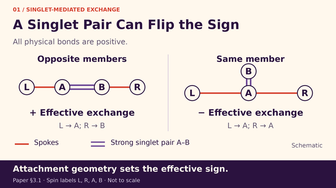
Electron hopping naturally supplies positive exchange, so signed couplings must first be converted. Insert a strongly coupled mediator pair and with bond strength . Its singlet has energy and its triplets have energy , leaving an excitation gap .
Attach the external spins to opposite pair members for positive effective exchange, or to the same member for negative exchange. Pauli correlations within one member of a singlet have the opposite sign from correlations across its two members. The second-order correction converts that sign difference into the desired coupling.
Quantitatively, for a penalty operator with kernel projection , complementary gap , and perturbation satisfying , Lemma 2 estimates the bottom energy using:
The inverse vanishes on the kernel, and the energy remainder is . Choosing polynomially large penalties controls it. Two further subdivision stages turn each spoke into a nine-link path, leaving the original central bond intact. All scalar energy shifts remain in the accounting.
For a source weight of magnitude , the spokes use strength . The two cross terms supply the factor of two needed to recover the desired interaction magnitude after division by the excitation cost. Increasing the penalty reduces the remaining error without requiring exponentially large coefficients. The effective energy also contains a computable scalar shift, which cannot be dropped when setting decision thresholds.
6. How Geometric Distances Encode the Required Spin Couplings
The positive-exchange model needs independently tunable distances. A rigid straight path would tie its edge lengths together, so the proof uses bent planar contact templates. Original lattice endpoints remain 17 units apart. Positive-source templates place the central pair at coordinates and . Negative-source templates use and .
Initially every actual link has length one and nonlinks are at least 1.4 apart. Bends make the fixed-end link-length differential surjective: small requested changes in every link length can be realized by moving internal vertices. A fixed-size contraction calculation computes those movements while keeping nonlinks more than 1.2 apart.
The layout is then enlarged by . Orbital overlap decays essentially exponentially with distance, turning these geometric adjustments into calibrated hopping strengths. Unwanted hopping between nonneighbors becomes small enough for the energy budget.
Each link requires solving a scalar equation: the actual hopping is , where is a positive overlap integral. Opposite signs at two nearby distance endpoints provide a bracket. Approximate bisection achieves the required residual without assuming monotonicity or a derivative bounded away from zero.
7. How Localized Electron Orbitals Produce Heisenberg Superexchange
Each of sites receives one localized spatial mode with two spin states, and the construction uses electrons. Let denote same-site Coulomb repulsion, direct repulsion between sites, and occupancy. In the finite model’s energy units, a positive quadratic occupancy penalty favors exactly one electron per site.
Long-range Coulomb terms cannot simply be discarded. Adjusting each well depth supplies a one-body counterterm with . Together, direct interactions and that counterterm become:
Here . A uniform positive lower bound on the Coulomb coefficient matrix gives nonzero integer occupancy defects a fixed energy cost. One electron hopping to its neighbor creates a doubly occupied site and an empty site, costing . Hopping back produces:
This is Heisenberg superexchange in Pauli normalization. Triplets do not hop into same-site pairs; the singlet receives the second-order energy lowering. Choosing reproduces positive target exchange scaled by . The small inverse-polynomial parameter suppresses higher-order errors.
8. Constructing the Coulomb Potential from Positive Nuclear Charge Density
The proof first designs a continuous positive density, then replaces it with nuclei. In dilated coordinates , dividing energies by leaves kinetic energy unchanged in form. Unit-nucleus attraction and electron repulsion acquire coefficients .
A broad uniform slab of density creates, near the modes, transverse confinement approximately after subtracting a constant. Compact planar wells provide localized modes. Their depths also supply the Coulomb counterterm. Calling the well contribution , Poisson’s equation identifies the required density:
Choosing a sufficiently large fixed background density keeps this quantity nonnegative, despite the local well modifications. The slab is finite, and its approximation errors are bounded both near the modes and outside them. Thus confinement is synthesized from attractive Coulomb charge, rather than added as an independent potential in the final input.
The reference orbital separates into a translated planar ground mode and a transverse Gaussian. The isolated planar well has energy −1/2 and a fixed gap above its mode. Its exponential tails control overlaps. Gaussian confinement controls vertical excursions. These explicit one-particle ingredients support the later continuum comparison; the proof does not assume that a chosen basis happens to approximate the answer.
9. Turning Continuous Charge Density into Unit-Charge Nuclei
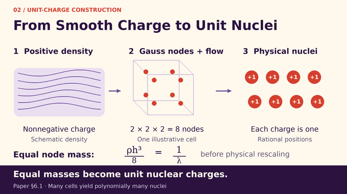
A smooth density transport moves uniform slab density into the designed density. The proof constructs the flow using a continuity equation. Because the flow transports measure, it moves quadrature nodes without changing their masses.
Each cube of side receives eight nodes: two Gauss points per coordinate, combined by tensor product. Each coordinate is the midpoint plus or minus . The rule integrates polynomials through total degree three exactly. Choosing the scales to satisfy the following identity makes every node equal in mass:
Transported node positions are rounded to distinct rational triples, with displacement small enough to control the Coulomb form error. Returning to physical coordinates multiplies the dilated charge coupling by , so each mass corresponds to physical charge exactly one.
The eight-node choice is consequential. Smooth orbital matrix elements receive fourth-order cubature accuracy, while arbitrary states near point singularities receive a weaker second-order form bound. A single undifferentiated approximation estimate would miss the mechanism that closes the proof.
The slab and node count can be enormous, but their exponents are fixed independently of the input. Rational rounding accuracy is also inverse polynomial, with the total nuclear mass included in its error budget. Polynomial-time implementability is an asymptotic statement here, not a claim that these configurations are convenient laboratory devices or efficient numerical benchmarks.
10. Proving That the Full Continuum Cannot Escape the Encoded Spin Problem
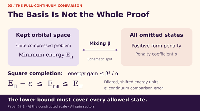
The deepest step is excluding a better answer elsewhere in continuous space. Let project onto the localized one-particle modes, including spin, and onto the many-electron space where every electron lies in those modes. The continuous one-particle operator has a fixed complementary gap. Small point-charge replacement errors preserve sufficient coercivity outside . This auxiliary gap differs from a molecular excitation gap, such as the spectral question in our Haldane gap explainer.
| Estimate | Scale And Role |
|---|---|
| Arbitrary-state form error | controls mixing in the form norm. |
| Compressed replacement error | directly controls orbital-space energy. |
| Complement elimination | follows by square completion. |
These scales use dilated, shifted energies. Here denotes a polynomial bound, source size, and . The polynomial may change between estimates. General form error is not a direct energy error: multiplying it by would leave an uncontrolled scale.
Instead, decompose a normalized state as , with and in the complement. The complementary penalty controls its first-order Sobolev norm, written . If is the remaining positive penalty and bounds mixing, square completion gives:
Thus mixing costs quadratically in , producing the smaller continuum correction. With the compressed minimum and the dilated, shifted Hamiltonian:
Positivity of electron repulsion helps retain the complementary lower bound. The mixed block is controlled in the Sobolev form norm, rather than by pretending the singular Coulomb potential is uniformly bounded. This distinction lets the argument apply to arbitrary allowed wavefunctions, including states concentrated near nuclei.
The upper bound tests states inside the mode space. The lower bound covers every antisymmetric form-domain state, uniformly in spin. This two-sided comparison, not orbital localization alone, transfers NO instances to the full continuum.
11. Completing the Hardness Proof: Error Bounds, Thresholds, and Limitations
After multiplying dilated, shifted energies by , Proposition 6 compares the continuum infimum with the finite fermion ground energy within . This includes additional matrix errors, so its exponent differs from the cubature exponents. Undoing dilation and tracking all scalar shifts gives an affine map from source spin energy to physical electronic energy, with positive slope .
The physical energy error is at most . Choosing leaves room to round thresholds rationally while preserving YES and NO answers and obtaining . Fixed-power scale choices, fixed-dimensional numerical integrations, and controlled flow evaluation keep nuclear count, coordinate bit lengths, and runtime polynomial.
For developers, the useful question is which additional structure makes a chosen workload manageable: geometry, state preparation, restricted correlations, or a different accuracy target. The theorem does not evaluate those possibilities. It specifies a demanding general input family against which universal solver guarantees must be judged. Demonstrated performance still requires instance-level calculations and an explicit error criterion.
The theorem requires neither neutrality nor binding, a molecular spectral gap, a ground eigenvector, or a lower-separation promise for nuclei. It does not classify ordinary molecular workloads or demonstrate failure of a particular chemistry method. Our AI-assisted semiconductor analysis illustrates the different evidence needed for practical calculations. Similarly, the QAOA expressiveness result concerns a specified optimization model, not a universal efficient solver.
QMA hardness of electronic structure therefore identifies what a general-purpose energy solver would have to overcome. Quantum hardware does not automatically make every quantum problem efficient. Follow Binary Verse AI for explainers that connect theorem statements, proof mechanisms, and verification scope, so each result becomes something readers can use and understand.
What does QMA-hardness of electronic structure mean?
It means that every promise problem in QMA can be reduced efficiently to the specified electronic ground-energy decision problem. QMA contains problems whose quantum witnesses can be verified efficiently with bounded error. The result establishes worst-case hardness, but does not assert membership in QMA or QMA-completeness.
Why didn’t earlier fixed-basis electronic structure proofs already solve the continuum problem?
Minimizing over a prescribed finite orbital basis can exclude lower-energy continuum states. A finite-basis minimum gives an upper bound on the unrestricted energy infimum, but transferring a NO instance also needs a lower bound on omitted states. OpenAI’s proof supplies that comparison over the full spinful fermionic continuum.
Why is the unit-charge restriction significant if hydrogen is easy to solve?
A single hydrogen atom is simple, but polynomially large, carefully arranged collections of unit-charge nuclei can encode complicated quantum spin interactions. The theorem concerns these constructed families of many-electron instances, rather than isolated hydrogen atoms or every ordinary hydrogen-containing molecule.
How does OpenAI’s proof encode quantum spin interactions using only nuclear positions?
It converts signed Heisenberg couplings into positive exchange through singlet mediators, realizes those interactions through virtual electron hopping, and calibrates hopping with orbital separations. A positive continuous charge density is then replaced by distinct unit-charge nuclei while preserving the required energy estimates.
How can the proof use localized orbitals without imposing a fixed orbital basis?
The orbitals are analytical tools constructed inside the proof, rather than restrictions supplied as problem input. A complementary one-particle gap, separate form and compression estimates, and a many-electron square-completion argument show that states outside their span cannot lower the relevant energy enough to alter the promised answer.
Does the threshold separation of at least one imply a molecular spectral gap or a bound ground state?
No. It separates the YES and NO decision thresholds. It is not an excitation gap between molecular energy levels. The theorem requires neither binding nor a ground-state eigenvector, and uses the spectral infimum even when no normalizable state attains it.
Does QMA-hardness mean quantum computers or established computational chemistry methods cannot calculate molecular energies?
No. The theorem establishes worst-case hardness for a general problem family. It does not show that ordinary molecular instances are always difficult or that particular computational methods necessarily fail. An efficient quantum algorithm for every promised instance would imply that all problems in QMA have efficient quantum algorithms; the theorem does not prove that such an implication is impossible.