
A conformal map can preserve every local angle while squeezing area savagely near a slit. The Brennan conjecture asks whether that distortion nevertheless obeys a universal integrability limit. OpenAI’s 31-page manuscript, dated September 24, 2026, proves the conjectured open interval: the derivative raised to any power strictly between four-thirds and four has finite area integral. Neither boundary smoothness nor a bounded domain is required.
Released in October, the argument subsequently received substantive mathematical validation and a shorter treatment from four specialists. Its central idea turns excessive boundary distortion into an impossible comparison between saddles and maxima. Here is the Brennan conjecture proof explained through the original paper’s logical steps, with its sharp endpoints and verification scope intact.
Table of Contents
1. Brennan Conjecture: The 1978 Problem That Defied Proof for 48 Years
A domain is a connected open region of the complex plane. Simply connected means that every loop can contract to a point within it. A conformal bijection is an angle-preserving, one-to-one holomorphic map with a holomorphic inverse.
Write for the unit disk. The theorem considers a conformal bijection , where the boundary of in the Riemann sphere contains at least two points. This excludes degenerate cases where such a disk parametrization is unavailable.
1.1. Brennan Conjecture Key Facts
| Feature | Verified Scope |
|---|---|
| Origin | James Brennan’s 1978 conformal-mapping problem. |
| Maps | Conformal bijections from suitable simply connected plane domains to the disk. |
| Area range | , with both endpoints excluded. |
| Boundary assumptions | No boundary smoothness or domain boundedness requirement. |
| Critical spectrum | . |
| Endpoint status | Both endpoint area integrals can diverge. |
| Manuscript | OpenAI, September 24, 2026; 31 pages. |
James Brennan’s 1978 question concerns the area integral of . The derivative’s magnitude measures local length magnification; its square measures local area magnification. Integrability asks whether the cumulative contribution remains finite, even where magnification becomes extreme.
One reassuring example is : change of variables makes the integral equal to , the disk’s area, even if the original region is unbounded. Brennan asks how far that guaranteed control extends in either direction.
An inward slit illustrates the danger: near its tip, a derivative can behave like an inverse square root of distance. The challenge is proving that arbitrarily complicated boundaries cannot collectively produce worse integrability inside the proposed interval.
2. What Did OpenAI Actually Prove About Brennan’s Conjecture?
The main theorem establishes
Here is ordinary planar area. The endpoints are excluded by counterexamples, rather than an unfinished estimate.
The analytical engine is a uniform bound on normalized inverse-square circular means:
It holds for every , every normalized univalent disk map , and . The constant depends on the chosen loss, not on the map. Normalization means and .
For an unnormalized map, replacing by reduces to this class. Its nonzero derivative at the origin contributes only a finite scaling factor, so normalization loses no generality.
Consequently, the universal integral means spectrum satisfies . “Sharp” identifies this exact limiting growth exponent. It does not remove the positive loss from the displayed uniform bound or make the endpoint area integral finite. A similar distinction between a sharp threshold and an arbitrarily small loss appears in our local smoothing explainer.
OpenAI’s October 6 mathematics release attributes the research collection to an internal frontier model. That disclosure does not establish that an ordinary consumer chat session can reproduce this proof.
3. Why Earlier Mathematical Approaches Could Not Reach the Sharp Bound
Classical distortion theory gives excellent pointwise control. For a normalized univalent map, its derivative cannot become small faster than a constant times the distance to the disk boundary. Taking the inverse square yields a crude circular growth exponent of two.
Brennan needs one. The gap concerns frequency: a large value at one angle says little about how much of the circle experiences it. Charging every angle for the worst possible distortion overestimates the bill.
The slit heuristic explains the upper endpoint locally: integrating the inverse square-root singularity to power against planar area converges exactly when . It cannot establish a universal bound for all boundary configurations.
Earlier work progressively improved the integrability range and connected it to derivative means. Pommerenke developed integral-means methods, Carleson and Makarov identified a linear spectral tail for sufficiently negative powers, and Bertilsson pursued derivative coefficient estimates. Weighted Bergman-space methods brought general spectral bounds closer to the target without reaching it.
The missing step was reaching the inverse-square threshold for every univalent map. Results for restricted families could not establish that universal conclusion. This attention to exact thresholds also matters in the Falconer distance problem, although its geometry and estimates are different.
4. How Inverse-Square Integral Means Reformulate the Original Problem
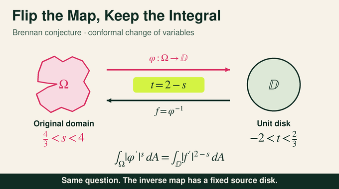
Let . The chain rule gives , while conformality supplies the area Jacobian . Therefore
Setting turns the desired range into . Negative powers detect small inverse-map derivatives; positive powers detect large ones. The substitution standardizes the source domain rather than assuming its boundary becomes regular.
The schlicht class consists of injective holomorphic disk maps with the normalization above. Define their circular averages by
The exponent and universal spectrum are defined by
This order matters: first compute each map’s asymptotic exponent, then take the supremum. The proof supplies the stronger uniform estimate directly. Normalizing a problem before attacking it is also a recurring theme in AI-assisted geometric proof discovery.
5. The Dyadic Transfer Operator: Turning Boundary Distortion Into Growth
The proof moves to the upper half-plane . Its compact normalized family contains univalent maps satisfying and . Compactness here concerns uniform convergence on compact interior sets.
Put . Changing the observation point to gives
The new map again belongs to . A positive operator averages observations at the two points , weighting each by . “Positive” means that nonnegative test functions remain nonnegative.
Explicitly, write and . These weighted base-point changes compose exactly, so the iterated derivative weights telescope rather than accumulating unrelated error factors.
Repeated application samples a dyadic grid at heights . Let denote the operator’s exponential growth rate. The paper proves that implies the required inverse-square radial estimate, using distortion bounds to compare grid samples with complete circular arcs.
The norm is taken over the whole normalized family, not one selected map. Once its growth rate is bounded, any number strictly larger than two controls all sufficiently long iterates up to a common multiplier. This is where the eventual uniform constant enters.
The threshold two has a concrete origin. After steps the boundary distance is comparable to ; growth like therefore corresponds to the desired reciprocal-distance exponent one. Subexponential allowances become the arbitrary positive loss.
The operator is an analytical construction. Unlike the program-search machinery discussed in our AlphaEvolve research explainer, it is not a reported numerical search algorithm.
6. The Probability Law That Makes Excessive Growth Contradictory
Assume instead that , and set . A positive eigenmeasure for the operator, followed by averaging horizontal translations and logarithmic scales, produces a probability law on .
For , its crucial weighted covariance identity is
It holds for every nonnegative Borel test function , meaning a measurable quantity attached to a sampled map. The derivative weight is essential: this is not ordinary translation invariance.
Taking the constant test function gives . Differentiate this identity to obtain moments of the logarithmic derivative :
The law is constructed only under the excessive-growth assumption. Showing it cannot exist eliminates that assumption for the entire compact family, rather than merely ruling out one candidate extremal map.
These exact expectations will determine a geometric sign. Probability organizes a hypothetical counterexample; it does not approximate the theorem through random trials. That role differs from studying an intrinsically random model such as percolation theory.
7. Why the Proof Needs Compact Superlevel Sets and Escape Estimates
Choose and a target . Define
At the possible preimage of the target, its value is infinite. Elsewhere it behaves like a landscape whose high regions can be counted.
But counting fails if peaks or saddles disappear toward the real axis or escape to infinity. The proof establishes that every positive closed superlevel set is compact inside the half-plane, for almost every sampled map and area-almost every target.
Weighted area estimates first control escape at positive heights. A further estimate bounds the total horizontal length mapped into a compact target region. At dyadic height , potentially troublesome targets can then be covered by disks whose total area is bounded by a constant times .
Those areas are summable across dyadic scales. The resulting exceptional target set has area zero. This technical step gives the later topological count somewhere safe to stand. It also makes clear why simply drawing a plausible landscape cannot replace the boundary estimates.
8. The Geometric Breakthrough: Pairing Saddles With Maxima
Away from its pole, the potential’s logarithm is strictly superharmonic: . It cannot have a local minimum. Its critical points satisfy
Define the normalized real Jacobian . For regular targets, positive Jacobian means a saddle and negative Jacobian means a maximum. This classification follows from the Hessian determinant and its negative trace.
The explicit identity linking analysis and geometry is
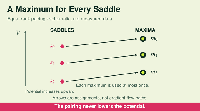
An index count on each compact superlevel component shows that maxima are at least as numerous as saddles above every positive height. A possible pole contributes its own index and must be counted separately. More precisely, components, maxima, saddles, and poles satisfy . There is at most one pole, and its component is present whenever it is, giving .
Order saddles and maxima independently by decreasing potential value, breaking ties lexicographically by coordinates. Pair equal ranks. Every saddle receives a distinct maximum at least as high. The assignment is measurable and respects affine source changes, allowing it to survive averaging.
Pairing equal ranks does not assert that a gradient-flow path joins the two points. It gives an injection within each target fiber, preserving enough order and symmetry for the area comparison. That modest requirement avoids demanding unnecessary geometry from the landscape.
The insight combines familiar tools in a productive arrangement. It is geometric bookkeeping, not a new rule of calculus. Readers interested in other concentration problems can compare our Kakeya geometry explainer, without treating that result as an ingredient here.
9. How the Jacobian Contradiction Completes OpenAI’s Proof
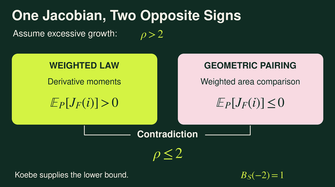
In the Jacobian identity, . Substituting the moments makes the linear and quadratic logarithmic-derivative terms cancel exactly. What remains has a strictly positive sign because :
Geometry now forces the opposite sign. The real area formula converts integration over source points into integration over targets, summing over their preimages. It applies separately to positive and negative Jacobian regions.
At a critical point, the relevant target weight is . The saddle-to-maximum pairing increases that weight. After averaging, affine covariance turns the source density into .
Expanding rectangular boxes make the relative cost of enlarging a box to contain paired points tend to zero. A separate area argument handles exceptional targets at the normalized root, where a generic-target statement alone would be insufficient.
Together these steps yield , contradicting the positive expectation. Thus , and the uniform inverse-square estimate follows. The force of the argument lies in deriving incompatible signs for the same quantity under the same hypothetical probability law.
10. From the Sharp Inverse-Square Bound to Brennan’s Full Integrability Range
For , write . Hölder’s inequality gives
Choose the positive loss small enough that . Radial integration is then finite. For example, permits , giving an integrable growth exponent of three-quarters.
The positive range needs a separate argument. Injective area change makes area-integrable for . Classical growth estimates and another application of Hölder supply the desired derivative powers. The factorization uses , possible exactly when , alongside integrability of . At , the integral is simply the disk’s area.
Sharpness comes from
Near minus one its derivative vanishes linearly; near plus one it has cubic blow-up. The endpoint powers both produce a logarithmically divergent radial area integral on suitable sectors. Thus and , equivalently and , genuinely fail.
For analysis researchers, the resulting derivative bounds also control certain pullbacks between homogeneous Sobolev spaces, where size is measured through gradients. They provide theoretical guarantees under rough geometry, without specifying a numerical solver’s conditioning, mesh requirements, or runtime.
11. How the Brennan Conjecture Proof Was Formalized and Mathematically Validated
OpenAI’s published Lean scope note covers the integrability interval, inverse-square spectrum, uniform radial estimates, and endpoint divergence. Corresponding solution proof modules are separate from comparator statement templates. This article does not report a fresh Lean build or a line-by-line formalization audit of the PDF.
Reproducing verification requires checking the encoded theorem, its imported dependencies, and the repository’s comparator configuration. Reading a scope note supplies a map of that work, not a substitute for executing it.
11.1. Evidence and Its Limits
| Evidence | What It Establishes |
|---|---|
| Original manuscript | Full integrability interval, inverse-square exponent, and Koebe endpoint obstruction. |
| Lean artifacts | Published scope and solution modules; no fresh kernel replay reported here. |
| Human follow-up | Shorter proof by Binder, Ivrii, Prause, and Smirnov; strictness details deferred. |
In their October 16 follow-up, Ilia Binder, Oleg Ivrii, István Prause, and Stanislav Smirnov validate the results and present a substantially shorter argument. They emphasize that the ingredients were familiar but their combination had escaped experts. Their detailed proof establishes for , where restricts the spectrum to bounded univalent maps. Their announced strict improvement for nonzero interior exponents has details deferred to another paper. It should not be retroactively attributed to the original manuscript.
For AI readers, the useful distinction is discovery, formalization, and mathematical understanding. Evidence-led AI science reporting needs all three. Our coverage of Fermat’s Lean formalization explains why those achievements differ. Research validation also asks more than an LLM math benchmark score can answer.
The Brennan conjecture proof establishes new mathematical control over conformal distortion, including consequences for Sobolev pullbacks. It supplies no measured speedup for AI training or simulation. Follow Binary Verse AI’s AI mathematical proofs coverage for explanations that keep theorem scope, verification, and practical performance distinct.
What is Brennan’s conjecture in simple terms?
It says that the derivative of a conformal bijection from a suitable simply connected plane domain onto the unit disk has a finite area integral when its magnitude is raised to any power strictly between and . No smooth boundary or bounded domain is required.
Has Brennan’s conjecture finally been proved?
Yes. OpenAI released its proof in October 2026 in a manuscript dated September 24. An October 16 preprint by Ilia Binder, Oleg Ivrii, István Prause, and Stanislav Smirnov validates the results and presents a substantially shorter argument. OpenAI also publishes Lean formalization scope and corresponding proof modules. This should not be confused with a claim that every exposition detail has been independently audited.
Why was Brennan’s conjecture so difficult to prove?
Classical distortion estimates bound how small an inverse-map derivative can become at individual points, but they do not adequately control its average inverse-power behavior around circles near arbitrary boundaries. The decisive issue was how frequently extreme distortion can occur.
What does the inverse-square integral-means exponent mean?
It is the sharp universal power-law growth exponent of the circular average of as the radius approaches one, over normalized injective holomorphic disk maps. The original uniform estimate retains an arbitrarily small positive exponent loss. The spectrum value does not assert finite area integrability at the endpoint.
What was the key mathematical innovation in OpenAI’s proof?
It combines a derivative-weighted probability law with an affine-equivariant, measurable pairing of saddles and maxima of a target potential. If inverse-square means grew too quickly, analytical moment identities would force a positive expected normalized Jacobian, while the geometric pairing and area formula force it to be nonpositive.
Why are 4/3 and 4 excluded from Brennan’s conjecture?
The interval is genuinely open. The Koebe function has a derivative that vanishes linearly near minus one and blows up cubically near plus one. Its disk area integrals diverge at powers and . The inverse map therefore gives divergence at and .
Was OpenAI’s Brennan conjecture proof formally verified in Lean?
OpenAI’s published scope documents formalization of the full integrability interval, the sharp inverse-square spectrum value, uniform radial estimates, and endpoint divergence, with corresponding solution proof modules in its repository. The linked comparator files are theorem templates, not the solution proofs. This article has not rerun Lean and does not claim a line-by-line formalization audit of every detail in the PDF.