
A formula with a million Boolean variables has more possible assignments than any computer could enumerate. The exponential time hypothesis says that, for worst-case 3-SAT, an exponential dependence on the variable count cannot be escaped. OpenAI’s October 25, 2026 manuscript presents an escape: deterministic, exact counting in subexponential time and polynomial space for every fixed clause width. Checking whether that count is positive also decides satisfiability.
The released Lean formalization establishes a weaker, still subexponential bound. Independent academic examination is being organized, and neither artifact demonstrates a production-ready SAT speedup. The advance is a new worst-case guarantee, built from shared linear measurements, interpolation, and tensor contraction.
Table of Contents
1. What Is the Exponential Time Hypothesis?
Let count Boolean variables and count clauses. ETH rules out a worst-case 3-SAT algorithm with running time times a polynomial input-size factor. Here means that the exponent divided by tends to zero. An exponential lower barrier is commonly written .
1.1. Exponential Time Hypothesis: Key Facts
| Item | Verified Scope |
|---|---|
| Research artifact | The Exponential Time Hypothesis Is False; OpenAI manuscript dated October 17, revised October 25, 2026. |
| Input | Fixed-width -CNF; declared variables, clauses; fixed . |
| Output and resources | Exact satisfying-assignment count; deterministic bit operations; polynomial working space. |
| Formalization | Canonical-input counting theorem; weaker exponent than Appendix D. |
| Research status | Public artifacts; independent examination being organized; practical superiority undemonstrated. |
Worst case means every formula must be covered, including deliberately difficult instances. It differs from the typical behavior studied in our random 3-SAT threshold explainer. A distributional transition and a universal runtime guarantee answer different questions.
2. The 3-SAT Problem: Why Boolean Logic Becomes Exponentially Hard
A literal is a variable or its negation. A clause ORs literals, and a conjunctive normal form, or CNF, ANDs clauses. In 3-SAT, each clause contains at most three literals. One false clause rejects an assignment, regardless of how many others are true.
This example fails precisely when . Its satisfying assignments, ordered as , are , , , , , and . Thus is satisfiable and .
Decision asks whether at least one assignment works. #3-SAT asks how many work. Exact counting supplies the decision answer immediately, while merely finding one witness leaves the count unknown. This distinction also separates finding a maximum matching from enumerating all perfect matchings. Exponentially many candidates alone do not prove hardness: a clever algorithm may avoid listing them.
3. The Previous Barrier: Why Earlier SAT Algorithms Could Not Refute ETH
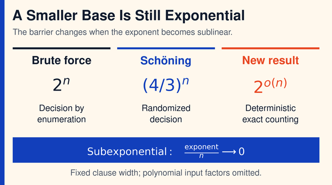
Earlier algorithms already beat brute force. Their achievement was reducing a constant exponential base, rather than making the exponent sublinear. The manuscript reviews local search, resolution-based guessing, and exact-counting methods as distinct starting points.
3.1. Earlier Algorithms And The Remaining Barrier
| Method | Guarantee And Qualification |
|---|---|
| Exhaustive search | assignments, with polynomial checking work. |
| Schöning local search | Randomized bounded-error 3-SAT decision in polynomial factors times . |
| PPSZ family | Uses bounded resolution and random variable ordering; historical and improved analyses reduce the exponential base. |
| Earlier fixed-width exact counting | Bounds of the form times polynomial factors, with algorithm-dependent randomness guarantees. |
For any fixed , : the exponent remains linear. A smaller base is valuable without contradicting ETH. Counting bounds cannot simply be substituted for decision benchmarks either, because the required output differs. The new result crosses this qualitative boundary by making the exponential-rate coefficient tend to zero.
4. The OpenAI Proof: A Deterministic Subexponential Algorithm For #k-SAT
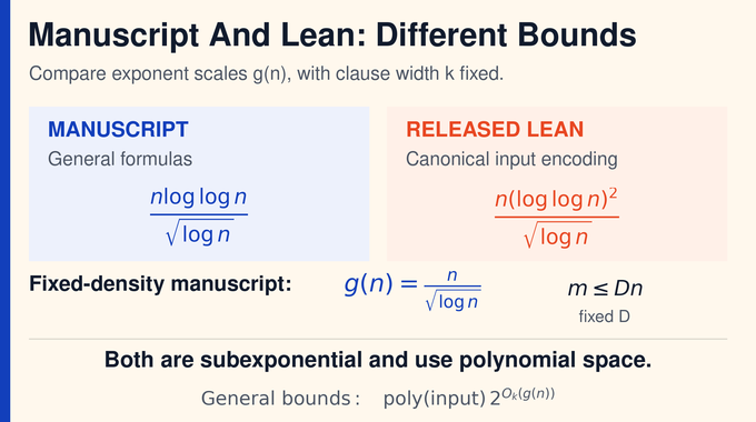
Theorem 1.1 in the revised manuscript states the general bound below, measured in bit operations. Constants hidden by the subscript depend on fixed clause width, rather than growing freely with the input.
For fixed density bound , inputs satisfying receive the stronger guarantee:
Both exponent ratios tend to zero. The theorem covers , with smaller cases handled directly, and uses bits of space. Logarithms in the manuscript are natural logarithms.
Computing and testing decides 3-SAT. Declared but unused variables remain important: each doubles the count. Fixed is essential. These guarantees do not authorize substituting a clause width that increases with .
Counts also support witness recovery. Fix one variable, count the remaining solutions, and retain a branch with positive count. Repeating yields a satisfying assignment. Choosing branches in proportion to their counts instead produces an exactly uniform random solution, with polynomial expected overhead. This is a consequence of exact conditional counting, distinct from the graph sampler in our switch-chain mixing explainer.
5. Turning Satisfying Assignments Into An Algebraic Counting Problem
The proof first illustrates its machinery on bounded-occurrence formulas. Represent false and true by zero and one. A positive literal becomes its variable, while a negative literal becomes one minus its variable. The clause below has an exact satisfaction indicator:
On Boolean inputs, this equals one precisely when holds. Multiplying all clause indicators rejects any assignment violating a clause. Summing over assignments therefore gives:
Here the index set contains the clause factors. This identity is not itself a speedup: direct summation still visits every assignment. Shared variables also prevent multiplying independent clause counts. Two clauses mentioning the same bit must agree on that bit. The algebraic translation resembles our Existential Theory of the Reals analysis, although this problem sums over Boolean assignments rather than searching real solutions.
6. Shared Linear Summaries: The Core Idea Behind Faster Counting
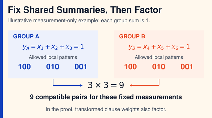
Partition the variables into small groups. If every clause stayed inside one group, local counts could be multiplied. Real formulas cross group boundaries, so the proof replaces their inputs with carefully designed linear forms at selected parameter values.
An integer measurement is a weighted sum of a group’s bits. For example, has four possible values. Fixing leaves three local assignments. Such a summary need not identify every bit to supply the information other groups require.
The construction arranges that a transformed clause reads its assigned group directly and other groups only through shared measurements. After fixing all measurements, group sums factor. Enumerating measurement tuples then restores the full total without double counting.
The tradeoff is precise: smaller groups reduce local enumeration, but too many summaries recreate exponential work. Summaries are shared across clauses, and their integer coefficients have bounded magnitude. At these transformed evaluation points, clause factors can take non-Boolean values. They are algebraic intermediates, not new satisfiable formulas.
7. Low-Degree Replacement Forms And The Matrix Construction
The replacements depend polynomially on a parameter . At , every original input is restored. At selected nonzero integers, the measurement structure enables factorization. Low degree matters because recovering a high-degree polynomial would require too much information.
An auxiliary rational matrix supplies the decomposition. The important small rank is that of , not necessarily itself. Here is the identity matrix. This correction depends on relatively few exceptional directions, which become measurements.
The remaining matrix entries connect incompatible groups at only a few evaluation points. Multiplying an entry by factors that vanish at those points removes the unwanted dependencies while preserving its value at zero.
Commuting coordinate-swap matrices provide a common eigenbasis. Interpolating alternating signs over a central interval makes most directions fixed, while binomial-tail estimates bound the exceptions. The construction must satisfy both constraints together: few measurements and low substitution degree. Either property alone would be insufficient.
A useful interpretation is that the matrix leaves most information untouched and exposes only a small exceptional component. The algorithm does not assume an arbitrary SAT instance naturally has low rank. It constructs an auxiliary object with the required structure, then transfers that structure to the replacement forms. Confusing a constructed property with an input promise would miss the proof’s central contribution.
8. Recovering The Exact Count With Hermite Interpolation
After substitution, let denote the sum of clause-factor products. Its value is the original count. Ordinary evaluations may not determine it cheaply enough, so the algorithm also recovers local Taylor coefficients.
The coefficient of in is a Hasse derivative at . Over the rationals, it equals the ordinary th derivative divided by . Sufficient coefficients across distinct points uniquely determine a polynomial of bounded degree. This is Hermite interpolation.
The difficult step is obtaining those coefficients while preserving group separation. The proof introduces separate formal variables for changes in the replacement forms. A coefficient of low Taylor order can involve only a correspondingly small number of these variables. Inclusion–exclusion then recovers the required sums from restricted evaluations.
Only truncated coefficient arrays are manipulated. The huge multivariate expansion justifies the identity but is never explicitly constructed. Exact rational arithmetic and coefficient-size bounds turn an algebraic operation count into an actual bit-complexity guarantee.
Why do derivatives determine the answer? If two candidate polynomials agree through several Taylor orders at a point, their difference has a root of corresponding multiplicity there. Adding those multiplicities across distinct points eventually exceeds the allowed degree. The difference must then be zero. Recovering the value at zero therefore requires no numerical approximation or floating-point extrapolation.
9. From Sparse Polynomial Equations To Arbitrary k-SAT
The illustrative occurrence restriction must now disappear. Counting-preserving sparsification partitions satisfying assignments among sparse leaf formulas on the original variables. Disjointness is crucial: adding overlapping leaf counts would overcount solutions.
Each clause has a violation polynomial over the two-element field. Its value is one for a violated clause and zero otherwise. Short parity tests combine these violation bits into polynomial equations.
Parity alone is insufficient because an even number of violations can cancel. Expander-code checks first ensure that any nonzero violation vector surviving the tests has many nonzero coordinates. Additional tests then eliminate all surviving nonsatisfying assignments.
The extra tests are chosen deterministically by comparing exact common-zero counts. A valid satisfying assignment passes every candidate, so minimizing the surviving count also minimizes unwanted assignments. Repeating the reduction removes them all. This use of a previously established polynomial-system counter avoids circular reasoning. Integer lifts and truncation modulo powers of two keep the combined degree manageable without changing the final exact count.
For intuition, a parity test on two violation bits accepts both zero violations and two violations. The code-based stage prevents small undetected patterns; the greedy stage handles the large ones. Neither stage alone is advertised as enough. Their combination preserves every genuine solution while shrinking the set of false survivors to nothing.
10. Tensor Contraction: How The Proof Achieves Its Sharper Runtime
Appendix D improves the interpolation route through Boolean tensor networks. An edge carries a bit, and a vertex assigns a value to each pattern on its incident edges. Contraction sums products of vertex values over every edge assignment.
Clause tensors enforce satisfaction. Equality tensors make copied occurrences of a variable agree. At fixed clause density, the resulting network has linearly many wires. For arbitrary density, sparse polynomial systems and degree-controlled monomial encodings introduce the additional double-logarithmic factor.
The contraction algorithm recursively deforms wire identifications and interpolates. Divisibility by powers of two limits which interaction terms can survive at the working precision. Smaller child networks are processed sequentially, with implicit tensor descriptions and polynomially bounded recursion storage.
The released Lean scope notes instead document time , where is canonical encoding length, and polynomially many visited tape cells. That weaker exponent remains sublinear. It must not be presented as formal verification of Appendix D’s sharper bounds. As in our Turing-machine space explainer, memory accounting is a separate obligation from runtime.
The modular calculation is exact because the answer lies between zero and . Knowing it modulo uniquely identifies that integer. This is an information bound, not an approximation guarantee. Likewise, discarding terms divisible by the working modulus cannot change the residue. These safeguards explain how finite-precision arithmetic can still return the full count.
11. Why The Proof Refutes ETH, SETH, Gap-ETH And #ETH
Exact subexponential counting contradicts #ETH directly and ETH through the positive-count test. It also contradicts the strong exponential time hypothesis: every fixed width now admits a subexponential algorithm, whereas SETH requires some fixed width to resist each specified constant improvement over exhaustive search.
Gap-ETH asks an algorithm to distinguish satisfiable formulas from formulas where every assignment violates a constant fraction of clauses. Exact satisfiability already distinguishes those promised cases. The deterministic algorithm also rules out the corresponding bounded-error randomized hypotheses.
11.1. Graph-Counting Consequences
| Task | Manuscript Guarantee |
|---|---|
| Independent sets | Exact deterministic counting in time. |
| Proper colorings | For each fixed , exact counting in time. |
| Perfect matchings | Exact deterministic counting in time. |
Here and count vertices and edges; all three guarantees use polynomial space. The perfect-matching exponent measures vertices plus edges, an essential qualification. Compare the different output guarantee in our perfect-matching approximation explainer.
Conditional implications remain valid mathematics when their assumptions fail. ETH-based optimality arguments lose that foundation, but unconditional results survive. Other assumptions may still support bounds discussed around edit distance and Subset Sum. A faster target algorithm requires a suitable reduction back to fixed-width SAT.
This distinction matters when reading older papers. A theorem saying that a faster algorithm would refute ETH has delivered exactly its promised implication. The new result changes which premise researchers can rely on, not whether the reduction was proved correctly. It also does not provide a blanket speedup for every problem previously studied under that premise. Parameter growth still has to be audited for each application.
12. What The OpenAI Proof Does And Does Not Establish
Subexponential does not mean polynomial. General polynomial reductions can enlarge the variable count enough to destroy a subexponential guarantee, so neither P = NP nor subexponential algorithms for every NP problem follow. Our shortest common superstring analysis likewise illustrates why approximation and exact optimization need separate guarantees.
For developers, the manuscript offers no benchmark establishing superiority over modern SAT solvers. Hidden constants, construction costs, and fallback cases matter. Even a polynomial theorem, as our three-machine scheduling explainer shows, can remain impractical.
OpenAI’s release announcement identifies an independent examination led by Russell Impagliazzo, Ramamohan Paturi, and Ryan Williams. As of October 27, 2026, that process should not be described as completed expert certification. This article checks the supplied manuscript and published scope notes; it does not report a local Lean rebuild.
The exponential time hypothesis result changes the theoretical question from whether this barrier can be crossed to how its algebraic machinery can be understood and improved. Follow Binary Verse AI for research explainers that keep theorem statements, formalization scope, and demonstrated performance distinct.
What is the Exponential Time Hypothesis?
The Exponential Time Hypothesis (ETH) states that 3-SAT requires exponential time in the worst case. It rules out algorithms running in time times a polynomial input-size factor, where is the number of variables.
How does the OpenAI proof refute the Exponential Time Hypothesis?
The manuscript constructs a deterministic subexponential-time algorithm that exactly counts satisfying assignments of fixed-width CNF formulas. A positive count means the formula is satisfiable, so the same algorithm decides 3-SAT within the stated bound.
Does the OpenAI proof mean P = NP?
No. Subexponential time is not necessarily polynomial time. The result contradicts ETH without establishing a polynomial-time algorithm for 3-SAT.
What is the difference between ETH and the Strong Exponential Time Hypothesis?
ETH excludes subexponential algorithms for 3-SAT. SETH states that, for every fixed positive improvement in the exponent over exhaustive search, some fixed clause width resists that improvement. The manuscript’s subexponential algorithm for every fixed width contradicts both.
Can the new algorithm solve large SAT problems efficiently in practice?
Not necessarily. The proved bound is not polynomial, and the manuscript does not demonstrate practical superiority over modern SAT solvers. Its primary significance is the new worst-case complexity guarantee.
Does refuting ETH invalidate previous computational hardness results?
Conditional theorems remain mathematically valid, but ETH can no longer support their hardness conclusions if its refutation is established. Some bounds may remain supported by different assumptions or unconditional proofs.
Has the Exponential Time Hypothesis proof been formally verified?
OpenAI released a Lean formalization of subexponential exact counting on canonical inputs. Its documented exponent, , is weaker than the revised manuscript’s sharpest bounds. As of October 27, 2026, independent academic examination is being organized. Lean verification should not be described as completed independent expert certification.