
An atom can attract an extra electron. Explaining why it cannot keep collecting them indefinitely is much harder. The Ionization Conjecture asks whether every atom has a universal ceiling on its excess electrons, however large its nuclear charge becomes. OpenAI’s September 24, 2026 manuscript presents a proof that a nucleus of charge strictly binds at most electrons, with one finite constant independent of the element. For molecules, the allowance grows with the number of nuclei. The paper also establishes separate bounds on neutral atoms’ first ionization energy and outer electron cloud. These are mathematical guarantees within a specified quantum model, rather than exact electron capacities for individual elements.
Table of Contents
1. Ionization Conjecture: How Many Extra Electrons Can an Atom Bind?
A neutral atom has as many electrons as units of positive nuclear charge. Adding electrons produces a negative ion if the enlarged system remains bound. Nuclear attraction competes with electron repulsion and the kinetic energy required by quantum mechanics.
The excess charge problem of atoms asks whether the number beyond neutrality stays bounded independently of nuclear charge. A bound proportional to charge would leave room for an ever larger surplus. A universal additive bound closes that loophole.
| Feature | Precisely Stated Scope |
|---|---|
| Quantum model | Full nonrelativistic Coulomb Hamiltonian, two electron spin states, fixed nuclei. |
| Molecular charges | Each nuclear charge is real and at least one; is their sum. |
| Excess electrons | At most beyond neutrality under strict binding, for nuclei. |
| Neutral atomic results | Uniform positive lower and finite upper bounds for first ionization energy and half-electron radius, for integer nuclear charge. |
| Publication status | September 24, 2026 preprint; independent verification is not established by the sources checked here. |
The 84-page research manuscript addresses that precise distinction. Its constant is not an element-specific prediction, and strict binding must be distinguished from a possible state at the dissociation threshold.
2. The Quantum Mechanics Behind the Ionization Problem
For electrons at positions , with fixed nuclei at distinct positions carrying charges , the Hamiltonian is
Here and . The Laplacian supplies kinetic energy. The negative potential attracts electrons to nuclei; the pair sum repels electrons. Atomic units fix the kinetic coefficient at one-half. Nuclear repulsion is omitted because fixed nuclei contribute the same scalar in every electron sector.
Wavefunctions are antisymmetric under exchanging complete position-and-spin labels, with two spin states. This Pauli constraint matters: the Bose–Einstein condensation problem concerns different particle statistics.
Write , the bottom of the spectrum, with . Strict binding means : adding the electron lowers the energy below the channel where it escapes. Equality alone does not exclude a threshold ground state. This is a nonrelativistic model without nuclear motion or applied magnetic fields.
3. Why Previous Proofs Could Not Establish a Universal Excess-Charge Bound
Lieb’s 1984 charge bounds gave linear control for atoms and molecules. Lieb, Sigal, Simon and Thirring later established asymptotic neutrality for fermionic atoms. Subsequent quantitative estimates reduced the allowed surplus further, but charge-dependent errors remained.
| Type of Result | What It Does and Does Not Establish |
|---|---|
| Linear charge bound | Caps electron count by a multiple of nuclear charge, with an additive term; permits a growing surplus. |
| Asymptotic neutrality | Makes the surplus a vanishing fraction of nuclear charge; does not make the surplus uniformly finite. |
| Hartree–Fock uniformity | Controls atomic ionization within the approximation; does not itself cover arbitrary many-body correlations. |
The distinction is elementary but unforgiving. A surplus growing like the square root of nuclear charge would become negligible as a percentage while remaining unbounded in absolute terms. Bulk accuracy cannot settle the last few electrons.
Solovej’s Hartree–Fock theorem established uniform atomic ionization bounds within that variational approximation. The full Schrödinger system permits correlations beyond a single Slater determinant. Extending screening control to those correlations is the central analytical difficulty.
The broader issue resembles the 2D area-law problem: useful energy information need not control the particular many-body quantity a conjecture asks about. Here that quantity is an additive electron count.
4. The OpenAI Proof: A Universal Bound for Atoms and Molecules
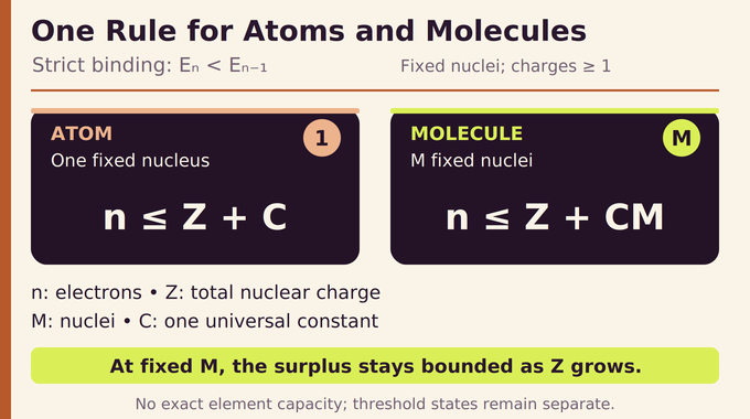
Theorem 1.1 states the molecular ionization conjecture in strict-binding form:
There are fixed nuclei, each with real charge at least one. The same finite constant works independently of their charges and distinct positions, including configurations with nuclei arbitrarily close together or far apart. Setting gives the atomic bound. Above the molecular ceiling, adjacent sector energies are equal.
OpenAI’s release announcement attributes the collection to an internal frontier model. That establishes provenance, not independent acceptance of this particular argument.
The supplied Lean scope document for result 263 describes companion asymptotic energy and radius theorems. It does not document complete formalization of this manuscript’s three headline conclusions. The sources checked here do not establish independent verification of this specific proof. That distinction follows the same principle discussed in our guide to AI mathematical proofs: identify the statement actually covered by each verification artifact.
5. First Breakthrough: Finding the Minimum-Energy Electron Sector
A local argument may need to remove electrons from an overcrowded region or insert them into an underfilled one. Insisting on one fixed total particle number makes those comparisons awkward.
The manuscript first proves the coarse bound for every strictly binding sector. Sector energies are nonincreasing: an extra electron can be placed increasingly far away, with negligible added energy. Since strict decreases cannot continue beyond the coarse ceiling, there is a largest strictly binding sector that attains the minimum over all particle numbers.
This common floor gives every admissible trial state the same energy benchmark, whichever integer sector it occupies. No convexity assumption about the sequence of sector energies is required.
The authors then define a delta-state as a normalized state with energy at most , where . The parameter tracks how far a modified state sits above the floor. Conditioning on an event or applying a spatial weight changes energy, so later estimates must tolerate this offset.
The initial bound is deliberately crude. Its purpose is to make the sharper local machinery possible, rather than supply the final excess-charge estimate.
6. Quantum Localization: Removing and Reinserting Trial Electrons
The localization step uses smooth spatial cuts, rather than pretending that electrons follow classical orbits. Squared cutoff functions partition probability between retained and removed groups. Their gradients generate an explicit kinetic localization cost, often called the IMS error.
Crucially, the construction records removed positions and spins. Conditional on those data, the retained core remains an antisymmetric quantum state. Its density determines a screened potential: nuclear attraction reduced by the core’s electronic repulsion.
Lemma 3.4 gives an exact energy identity. It accounts for the conditional core energy, removed-particle kinetic energy, attraction through that screened field, mutual repulsion among removed electrons, and localization error. Keeping the conditional field preserves information that replacing the core by an unconditional average would lose.
Next, the proof inserts localized trial orbitals into a spatial hole, separated from the core. Antisymmetrization respects Pauli exclusion, while separated supports make the energy comparison manageable.
The trial construction allows a noninteger expected particle count by averaging over genuine states with integer counts. Every realization still lies above the common energy floor. Nothing divides a physical electron.
This is the key logical exchange: compare the actual local population with flexible alternatives, yet retain valid fermionic states and account for every energetic cost. The proof gains freedom across sectors without relaxing the underlying many-electron model.
7. Thomas–Fermi Screening: The Mathematical Engine of the Proof
Thomas–Fermi theory replaces detailed orbitals with a density description. Here it supplies a local comparison functional, while the state being bounded remains fully quantum and correlated.
The Lieb–Thirring kinetic inequality first prevents excessive density concentration. Its positive coefficient is sufficient for coarse control, but the manuscript explicitly does not identify it with the exact Thomas–Fermi coefficient.
That coefficient comes from separate constructions: coherent-state filling provides an upper trial comparison, and Neumann eigenvalue counting in small cubes provides a lower comparison. Explicit remainder terms accompany both. Matching their leading kinetic coefficients lets the proof compare the same convex functional from opposite directions. If those coefficients differed by a fixed amount, their mismatch would multiply a density integral that grows with nuclear charge. An apparently modest discrepancy could therefore swamp the few-electron information being sought. Explicit control of the remainders is as important as identifying the leading term.
For its local minimizing density and screened field,
Here . Positive screened attraction supports density; the positive-part operation suppresses the response where that attraction is absent. This relation is a comparison law, not an assertion that the exact electron density equals the Thomas–Fermi density everywhere.
The resulting estimates control local electron-count second moments and Coulomb discrepancies between densities. Second moments matter because a small mean can conceal rare, heavily crowded configurations. Those configurations cannot simply be discarded when the proof later conditions on observations.
Screening therefore becomes quantitative and stable under energy offsets, supplying the link between local quantum mechanics and the outward field argument.
8. Noisy Observations and Conditional Screening: Controlling Electron Correlations
The proof introduces artificial noisy observations of electron positions. Independent errors blur the positions at a chosen width, and particle labels are forgotten. These are auxiliary probability constructions inside the argument, not measurements performed on an atom.
For an observation event of probability , multiplying the wavefunction by the normalized square root of its likelihood produces an antisymmetric conditional state. Lemma 5.2 bounds the extra energy by
The width controls observation precision, and is the base of natural logarithms. For the specified noise law and scale arrangement, the constant carries no factor proportional to electron number or the number of observation arrays. Sharper observations cost more kinetic energy; rarer events increase the logarithmic penalty.
That dimension-free feature is essential. A cost growing with electron count could destroy the universal additive estimate sought at the end.
Conditional smoothed densities generate screened fields. A proposed failure of their local Thomas–Fermi comparison can be tested by applying the quantum estimates to the corresponding conditional state. The argument also controls rare negative-field configurations that could spoil averaging.
One subtlety deserves emphasis: the original observation posterior and the posterior after making a fresh spatial cut are different laws. The proof uses separate conditional-expectation identities to transfer estimates between them. Correlations remain present throughout. As in the quantum Heisenberg ferromagnet argument, conditioning is useful only when its changed probability law is accounted for.
9. Outward Propagation: How the Proof Finally Bounds Excess Electrons

Local screening is not yet a global charge bound. The proof must transport its control through increasingly large spatial scales without accumulating an error proportional to nuclear charge.
A positive comparison field starts near the nuclei. At each scale, a local maximum selects between a shifted nonlinear comparison field and a shifted observed field. The shifts create room for the inverse density-field estimates to justify whichever branch wins.
This construction replaces the model’s nonlinear response by the actual conditional electron density through one additional spatial layer. Only afterward does conditional averaging forget the current observation array. Convexity preserves the required inequality under that averaging.
Failed comparisons contribute a nonnegative error density. The proof sums its expected spatial integral. It does not demand one observation outcome that behaves well simultaneously at every spatial point. This avoids an unnecessarily expensive global exceptional-event estimate.
Molecular geometry adds another challenge: large regions can contain no nuclei across many successive scales. A hierarchy of nuclear representatives controls those voids with total cost proportional to the number of nuclei, without paying separately for every empty scale.
Finally, a potential comparison and spherical averaging relate the positive exterior field to nuclear charge minus enclosed electron mass. An exterior electron-count estimate controls what remains outside. If excess charge per nucleus could grow without bound, these estimates would contradict one another.
That contradiction supplies the uniform excess charge bound. It is an existence theorem for a finite constant, rather than a calibrated rule saying which particular negative ion a laboratory can prepare. The spatial cuts used here also differ from physical disorder-induced trapping in Anderson localization.
10. First Ionization Energy: Why Removing One Electron Has a Universal Energy Bound
For a neutral atom with integer , write for the energy with electrons. Corollary 1.3 states
Energy is measured in the paper’s atomic units. The constants are independent of nuclear charge and need not match constants elsewhere in the argument.
The positive lower bound does not say that different atoms have the same ionization energy. It says the whole sequence stays away from zero, while the upper bound prevents unlimited growth.
This first ionization energy bound has its own atomic proof. The molecular excess-charge theorem is not used to derive it. Shared screening tools first establish an interior electron deficit for suitable atomic sector ground states.
Deleting exterior particles then places neutral and singly ionized ground states within a bounded energy offset of the global sector minimum, giving the upper bound. An averaged insertion trial in the singly ionized atom exploits its residual positive charge. Controlling the hole’s kinetic cost and discarded configurations produces a uniform positive lower gap.
This gap compares different electron sectors. It is distinct from the within-sector excitation gap discussed in the Haldane gap conjecture. Neither bound calculates element-specific spectroscopy or demonstrates faster electronic-structure software.
11. The Outer Radius of Neutral Atoms: Why Electron Clouds Remain Controlled
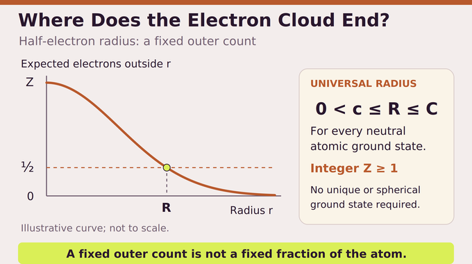
Let be the spin-summed density of any normalized neutral atomic ground state. Its integral is . The paper defines
This half-electron radius describes expected exterior electron mass. It neither divides an electron nor marks a sharp boundary of the cloud. Theorem 1.2 places it between positive universal constants, without assuming a unique or spherically symmetric ground state.
The lower radius estimate follows from the atomic deficit argument: enough density remains outside a fixed small radius. For the upper estimate, the positive ionization gap combines with shell weights and conditional screening to bound the large-radius tail by a constant divided by radius. Finitely many smaller nuclear charges are handled separately.
Bulk density lives on the shrinking Thomas–Fermi length scale . The half-electron criterion follows a fixed exterior mass whose fraction of the whole atom tends to zero. Bulk convergence therefore cannot establish this outer-radius conclusion.
The Ionization Conjecture manuscript’s contribution is this coordinated control of surplus charge, removal energy and outer density within the stated model. It supplies analytical constraints, without a demonstrated simulation speedup. Follow Binary Verse AI for research explainers that trace ambitious theorem statements back through their assumptions and actual proof mechanisms.
How many extra electrons can an atom hold according to the OpenAI proof?
For an atom with nuclear charge , Theorem 1.1 bounds the number of strictly bound electrons by , where is a universal finite constant. It does not give the exact maximum number of extra electrons for each element.
Has the ionization conjecture finally been proved?
The September 24, 2026 OpenAI manuscript presents a proof of the excess-charge conjecture in its strict-binding formulation for the full nonrelativistic two-spin Coulomb model. It does not exclude every possible threshold ground state. The sources checked for this article do not establish independent verification of this specific manuscript, and the supplied Lean scope note covers companion asymptotic results.
Why was the ionization conjecture so difficult to solve?
Earlier estimates could constrain electron numbers or prove that atoms become approximately neutral at large nuclear charge, while still allowing an unbounded surplus. Obtaining a uniform additive bound required controlling local electron densities and screening in the fully correlated quantum system without errors growing with nuclear charge.
How does the OpenAI proof improve upon Hartree–Fock theory?
Solovej’s Hartree–Fock work established uniform atomic ionization bounds within that variational approximation. The new manuscript addresses the full many-electron Schrödinger Hamiltonian, admitting correlations beyond a single Slater determinant. This extends the mathematical scope; it does not demonstrate improved numerical accuracy or faster simulations.
Does the OpenAI proof apply to molecules as well as atoms?
Yes. For fixed nuclei at arbitrary distinct positions, each with a real charge of at least one and total charge , Theorem 1.1 gives whenever the -electron sector binds strictly. The same finite constant is independent of nuclear charges and positions.
What does the proof establish about the first ionization energy?
For neutral atoms with integer nuclear charge , Corollary 1.3 defines and gives . Thus the first ionization energy has a positive universal lower bound and a finite universal upper bound in the stated nonrelativistic two-spin model and atomic units. This is a separate atomic argument using shared screening estimates.
What is the half-electron radius in the OpenAI proof?
It is the infimum of radii outside which the expected electron density integrates to at most one-half electron. Theorem 1.2 bounds this radius above and below by positive universal constants for every normalized neutral atomic ground state with integer nuclear charge. It describes an expected exterior electron count, not a physically divided electron or a sharp edge of the cloud.