
A computer can count every satisfying assignment of a finite Boolean formula and still lack a guaranteed way to calculate the transition point of infinitely growing random formulas. OpenAI’s September 27, 2026 preprint closes that gap for the random 3 sat threshold: one deterministic program can approximate the limiting critical ratio to any requested accuracy. It does not calculate the famous predicted value near 4.267, establish a practical runtime, or solve arbitrary 3-SAT instances quickly. The advance is a pair of finite certificate searches that trap an infinite-system constant between increasingly tight, justified bounds.
Table of Contents
1. Random 3-SAT Threshold: When Do Random Formulas Become Unsatisfiable?
A Boolean variable is true or false. A literal is a variable or its negation. A 3-CNF formula joins clauses with AND, while each clause joins three literals with OR. Satisfiability asks whether one assignment makes every clause true.
For example, is satisfied by setting all three variables true. It has three variables and two clauses, so its density is . This illustrates the notation, not a threshold estimate.
| Item | Verified Scope |
|---|---|
| Research source | OpenAI preprint, September 27, 2026. |
| Random model | Three distinct variables per clause, independent fair signs, independently sampled clauses; repeated clauses allowed. |
| Main result | The limiting threshold is a computable positive real. |
| Accuracy | Rational output with absolute error at most for every integer . |
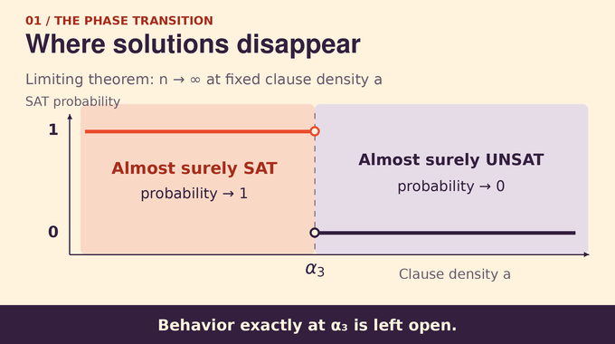
| Limits | No numerical evaluation or efficiency estimate; behavior exactly at the threshold remains open in this theorem. |
For , the model samples uniformly from possible clauses, with replacement. Write for the probability that the resulting formula is satisfiable. Probability concerns the random formula, unlike the worst-case input guarantees examined in our trace reconstruction analysis.
2. Why the 3-SAT Critical Ratio Is Predicted Near 4.267
Adding clauses removes possible assignments. At sufficiently low density, almost every large random formula is satisfiable. At sufficiently high density, almost none is. The 3-SAT phase transition concerns that collective change, rather than a rule deciding each individual formula.
For ten thousand variables, forty-two thousand clauses give density 4.2. That arithmetic alone cannot classify the formula. The limiting statement concerns repeated random draws as the variable count grows, rather than certainty at a particular finite size.
Statistical-physics calculations using the cavity method predict a transition near 4.267. They model the organization of satisfying assignments and its evolution as constraints accumulate. The prediction has guided research, but the phrase “random 3 sat threshold 4.267” must not turn an approximation from physics into an exact proved constant.
Rigorous bounds answer a narrower question: which densities can be certified below or above the transition? A separate October 2026 preprint by Fedor Vorobyev reports an upper bound of 4.268. That statement is distinct from proving equality with the cavity prediction. OpenAI’s computability manuscript does not supply a numerical evaluation.
Our percolation theory explainer makes a related distinction between locating a critical point and understanding behavior there. For random 3-SAT, this theorem specifies probabilities strictly on either side, leaving equality untreated.
3. The Previous Barrier: A Sharp Transition Was Not Enough
Friedgut’s sharp-threshold theorem showed that the transition narrows around a location depending on formula size. Narrowing does not force that location to converge. A very precise needle can still move across the dial.
Gaia Carenini’s polynomial scaling-window paper establishes limiting thresholds for every fixed clause size of at least three, combining its window estimate with a result of Abbe and Montanari. OpenAI explicitly credits Carenini with priority for resolving the existence conjecture. Its own probability argument also constructs the three-clause limit because the computability proof needs additional quantitative information.
Ding, Sly, and Sun had previously proved existence and the statistical-physics characterization for sufficiently large fixed clause sizes. That result did not automatically cover three literals.
Existence, computability, and computational cost are separate achievements. Our Existential Theory of the Reals analysis similarly distinguishes a problem’s decidability from stronger resource bounds. Here the central question is whether any finite program can reliably produce arbitrarily accurate approximations to one limiting real number.
4. What the OpenAI Proof Establishes About the Random 3-SAT Threshold
Theorem 1.1 of Computing the Random 3-SAT Threshold identifies a positive finite number . For every fixed nonnegative density , the statement is:
The floor brackets mean taking the integer part, since clause counts are integers. Separately, one finite deterministic Turing machine takes a unary precision request , meaning a string of ones, and halts with a rational output satisfying:
The program receives no oracle, hidden real constant, or advice. Its task is numerical approximation of a distributional boundary. It does not decide arbitrary satisfiability instances or remove the NP-completeness barrier associated with 3-SAT. As in our time-space tradeoff explainer, the computational resource being guaranteed matters: eventual termination says much less about speed than a runtime estimate would.
OpenAI places the manuscript in its AI mathematics release. The published Lean scope note reports coverage of threshold computability. Its comparator configuration points to a separate solution module, rather than treating the comparator’s placeholder as a proof. We have inspected those materials, not independently rebuilt the Lean development. Formalization scope and mathematical review remain separate questions.
Although the surrounding existence results cover other fixed clause sizes, this computation theorem concerns three literals. Extending the same computability conclusion requires its own argument.
5. Why Convergence Alone Cannot Make a Threshold Computable
For each finite size, exhaustive enumeration can determine satisfiability probabilities. Why not increase the size until the answers stabilize? Because apparent stabilization supplies no certified stopping rule. A later term might move farther than the requested error permits.
Specker’s classical example shows that even a bounded, increasing, computable sequence of rational numbers can converge to a noncomputable real. Computing every term does not guarantee that a program can tell how near a term lies to the limit.
This is the distinction between computability and noncomputability underlying our Turing degrees explainer. A convergence proof may establish an answer’s existence while withholding the information necessary to approximate it on demand.
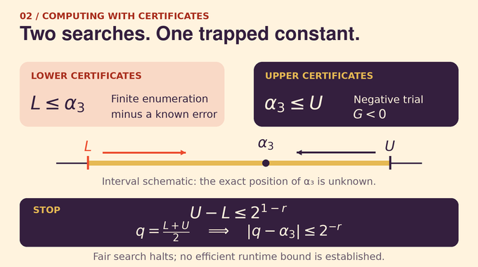
The new 3-SAT threshold proof supplies finite evidence from both directions. Lower certificates never exceed the true threshold and eventually approach it. Upper certificates occur at every rational density above it. Once two certificates leave a sufficiently short interval, the program can stop safely. It never needs to recognize convergence by watching a graph flatten.
A lower sequence by itself leaves an asymmetric problem: a computed value may be valid without revealing how much threshold remains above it. The upper family closes that gap with independently justified evidence.
6. The Poisson Model and the First Unsatisfiable Formula
The proof changes the sampling machinery temporarily. Clauses arrive according to a rate-one Poisson process. At time , their count has a Poisson distribution with mean . Each of the three variable positions is sampled independently, allowing repeated variables within a clause.
Let be the first arrival time at which the formula becomes unsatisfiable. Define its capped expected value:
The cap prevents extreme survival times from overwhelming the estimates. It is not a claim that the critical density is twenty. The proof establishes that normalized capped expectations converge to the threshold.
Poissonization is useful because disjoint categories of arriving clauses form independent streams. The proof can separate clauses touching a chosen variable from those avoiding it, then compare their effects without introducing dependencies between the streams.
One auxiliary low-density argument uses Hall’s theorem to assign clauses distinct representative variables, then sets those representatives to satisfy their clauses. This connects feasibility to the pairing structure introduced in our maximum cardinality matching explainer.
The model change requires justification. Removing clauses with repeated indices produces the proper-clause stream. Monotonicity, Poisson concentration, and comparisons at densities separated by fixed positive slack transfer the strict-side limits to exactly the original independently sampled, distinct-variable clauses. Simply calling the models approximately equivalent would omit a necessary proof step.
7. Free-Deletion Bounds, Concentration, and Weighted Interpolation
Imagine deleting one variable together with every clause touching it. How much longer can the formula remain satisfiable? The key estimate bounds the six-fifths moment of that extra capped survival time by a universal constant. Crucially, it still works when other variable deletions are already permitted.
The proof compares the surviving assignments under shorter tests and fresh three-literal clauses. Independent variable positions make the relevant killing probabilities exact powers. The analysis controls the entire residual candidate set rather than following one promising assignment.
This deletion estimate gives concentration: the moment of the capped time’s deviation from its mean grows at most linearly with . Its corresponding fluctuation scale is , which becomes negligible after dividing by .
Concentration alone does not compare different sizes. Weighted interpolation joins two independent blocks, allowing different clause densities, and compares their survival probabilities with the combined system. A weight-balancing argument then restores uniform sampling. The resulting error in the mean is sublinear.
Merging blocks through a dyadic construction makes the normalized errors summable. That yields convergence and, more usefully for computation, an explicit inequality valid at every finite size.
These are probabilistic estimates over random formulas, not uniform promises about every clause sequence. Keeping that distinction prevents a concentration theorem from being misread as a worst-case SAT algorithm.
8. How the Proof Constructs Certified Lower Bounds
The finite-size estimate supplies the lower half of the random 3 sat threshold formula:
The enormous constant and slow decay matter. This is a rigorous certificate, not a recommendation for numerical work. Even evaluating the finite expectation can require vast computation.
The inequality is one-sided. It tells us that subtracting the correction cannot overshoot the limit. It does not bound the absolute difference between the finite expectation per variable and the threshold, so it cannot replace the upper-certificate search.
At fixed size and clause count, enumerate every ordered signed clause list and all assignments. The satisfiability probability is rational. In the relaxed model, there are ordered lists of clauses. Weight these probabilities by the Poisson law and integrate survival up to the cap.
The infinite sum is not swept under the rug. An explicit Poisson-tail bound controls truncation, and certified rational intervals enclose the remaining exponential terms. Rational bisection also encloses the sixth root appearing in the correction.
Rounding downward produces rational lower certificates converging to the threshold. Unlike the efficient approximation guarantee discussed in our counting perfect matchings analysis, this enumeration establishes computability without a useful cost bound. Finiteness is doing the work here, not speed.
9. Robust Unsatisfiability and the Soft-Pressure Method
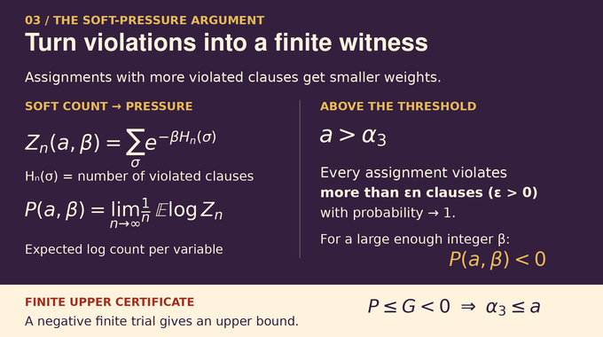
An unsatisfiable formula might miss satisfiability by only one clause. That is insufficient for the upper search. The proof needs robust failure: above the threshold, every assignment violates a positive multiple of the number of variables, with probability tending to one.
The deletion estimate supplies that strength. If an assignment violated only a small number of clauses, deleting one variable from each violation would remove them all. But above the threshold, the proof shows that even a sufficiently small linear allowance of variable deletions cannot restore satisfiability.
Let count violations by assignment , and let penalize each violation. The softened count is:
A satisfying assignment contributes one. An assignment with violations contributes a smaller positive weight. Define the pressure as the limiting expected logarithm per variable:
Interpolation proves that this limit exists. Below the threshold it is nonnegative for every finite positive penalty. Above it, robust violations overcome the exponential number of assignments, making the pressure negative for some positive integer penalty. That sign supplies something finite trials can certify.
The balance is explicit: . A positive density of unavoidable violations allows a sufficiently large fixed penalty to dominate the assignment-count term. Unsatisfiability by a single clause would not provide that linear margin.
10. Hierarchical Interpolation: Constructing Upper Certificates
A trial description contains finite rational averaging parameters and a finite table of message pairs in . The coordinates correspond to the two literal signs and need not sum to one. A finite hierarchy organizes conditional sampling and averaging.
The trial value is uniformly computable. Interpolation proves the upper bound . For the enumerable rational trial family, completeness gives:
The bound uses a nonnegative cubic remainder, , for nonnegative . Completeness is harder: trials obtained from finite formulas initially contain unwanted randomness shared across sites beyond the root.
The structural argument removes that nonroot sharing while controlling the change in trial value. Root randomness remains shared. Conditional-law records and Gaussian tests keep the descriptions valid under later changes of sampling law. A depth-independent estimate allows approximation tolerances to be fixed before the structural reductions finish.
Finally, independent site sampling and rational discretization produce finite tables. Some existence arguments choose subsequences non-effectively. That is permitted: the program receives no chosen limiting law. It searches every finite description and eventually encounters a witness whose existence the argument proves.
Evaluating a description still involves Poisson counts, exponentials, and logarithms. Certified tail truncations and rational enclosures control those operations. The search certifies negativity only when the entire enclosing interval lies below zero, avoiding an unreliable floating-point sign test.
The infimum identity is essential. If pressure is negative, sufficiently accurate trials must also be negative. An upper-bound inequality without completeness could leave every searchable trial positive, even when the true pressure was below zero.
11. How Both Certificate Searches Make the Threshold Computable
| Certificate | Finite Evidence | What It Guarantees |
|---|---|---|
| Lower | A downward-rounded finite expectation minus its explicit error. | A rational number below the threshold; such bounds approach it. |
| Upper | A trial-value enclosure with strictly negative upper endpoint. | The tested density is at least the threshold; every larger rational density has a witness. |
Start with the valid interval from zero to twenty. A fair schedule enumerates lower certificates, rational densities, integer penalties, finite trials, and evaluation precisions. Each successful certificate tightens an endpoint. The search does not wait forever on a trial whose value might equal zero.
For requested precision , it stops when interval width is at most and outputs the midpoint. The resulting error is at most . Termination follows because the lower certificates approach the threshold and every rational density above it eventually supplies a negative upper witness.
No computable rate of finite-size convergence is required. For developers, this establishes a possible certified computation, not a competitive threshold calculator. The manuscript provides no efficiency estimate, unlike an explicit runtime theorem such as the one discussed in our mean payoff games analysis.
The random 3 sat threshold is therefore computable in the precise sense that each requested approximation eventually arrives with a guarantee. Its numerical evaluation, practical cost, and behavior exactly at criticality remain separate tasks. Follow Binary Verse AI for research explainers that trace the mechanism behind a theorem and keep its guarantees visible.
What is the random 3-SAT threshold?
It is the limiting clause-to-variable ratio separating two regimes for independently sampled, uniformly signed clauses on three distinct variables. Below it, satisfiability probability tends to one as the number of variables grows. Above it, that probability tends to zero.
Is the random 3-SAT threshold exactly 4.267?
This paper does not establish that value. Approximately 4.267 is a statistical-physics prediction. OpenAI proves that the limiting threshold is computable without evaluating it numerically or identifying it with that prediction.
How does the OpenAI proof compute the threshold?
It constructs computable lower certificates and an enumerable family of upper certificates. A fair search through both families produces arbitrarily narrow rational intervals guaranteed to contain the threshold, then returns their midpoints.
Why wasn’t proving the threshold exists sufficient?
A real number can be the limit of a computable sequence without itself being computable. Existence and convergence alone may provide no effective stopping rule. The proof supplies finite certificates from both directions that overcome this obstacle.
Does the OpenAI proof solve the NP-complete 3-SAT problem in polynomial time?
No. It approximates a limiting threshold for a specified random-formula model. It does not give a polynomial-time algorithm for deciding whether arbitrary 3-SAT formulas are satisfiable.
Can the new algorithm efficiently calculate the threshold to many decimal places?
Efficiency is not established. The paper proves that one deterministic algorithm halts at every requested precision, but supplies no efficiency estimate or demonstrated practical runtime.
What happens exactly at the random 3-SAT threshold?
Theorem 1.1 establishes limiting satisfiability probabilities at fixed densities strictly below and strictly above the threshold. It makes no assertion about probability behavior at the threshold itself.