
An interacting quantum gas can look well behaved in every small region while still withholding the one thing a condensation proof needs: coherence across the whole sample. The difficulty grows with the box. A bound that works for a thousand particles may disappear when their number becomes unlimited.
The Bose Einstein condensation proof in OpenAI’s October 5, 2026 preprint addresses that problem for a three-dimensional dilute hard-sphere gas. It establishes a positive condensate fraction at a strictly positive temperature, with exclusion distance, density, and temperature held fixed as volume grows. Its central mechanism converts local control into a long-distance overlap bound whose cost depends on encounters between comparison routes, rather than their lengths.
Table of Contents
1. What the Bose–Einstein Condensation Proof Establishes
The research manuscript concerns the exact canonical Gibbs state, the equilibrium density operator for a fixed number of interacting bosons. It does not replace that state with an effective wave equation or assume condensation before analyzing excitations.
| Feature | Exact Setting |
|---|---|
| Model | Three-dimensional continuum gas with periodic boundaries and hard-core exclusion. |
| Density | Sufficiently small, fixed positive density for each fixed exclusion distance. |
| Temperature | A strictly positive value chosen independently of volume. |
| Equilibrium state | Exact canonical Gibbs state, with particle number fixed in each finite box. |
| Conclusion | Positive limiting lower bound on the fraction occupying the constant orbital. |
| Boundary of result | No transition-temperature calculation, complete-condensation theorem, or superfluidity conclusion. |
Let be particle number, the box’s side length, and the limiting density. Write for the one-particle density matrix, normalized to trace . The theorem establishes
Here is the normalized constant orbital. The fraction remains bounded away from zero along every sequence with the stated limiting density. The theorem does not assert that the fraction converges to one particular value.
OpenAI included the manuscript in its October mathematics release. That identifies its provenance. The evidence to examine is the argument and its assumptions, as in our broader guide to AI mathematical proofs.
2. The Original Problem: An Interacting Gas That Keeps Growing
The hard-sphere Bose gas lives in a periodic three-dimensional box. Opposite faces connect, removing boundary walls from the problem. Two particle centers must remain farther apart than the exclusion distance . Configurations violating that condition are forbidden, and the wavefunction satisfies a Dirichlet condition at the excluded boundary.
Inside the allowed configuration space, the Hamiltonian is kinetic energy. The interaction enters through the forbidden configurations, rather than a small bounded potential. The paper uses units with , where is particle mass and is Boltzmann’s constant.
Diluteness means the dimensionless gas parameter is sufficiently small. It does not mean interactions disappear as the box expands. The Bose gas thermodynamic limit takes and to infinity while approaches fixed positive density.
First choose the physical gas and an allowed positive temperature. Then enlarge it indefinitely. A temperature forced toward zero as volume increases would answer a different question.
3. What Actually Condenses: One Orbital, Many Correlated Particles
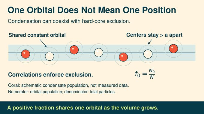
The one-particle density matrix records single-particle occupations and coherence after the other particles have been traced out. Its eigenvectors are natural orbitals. Bose–Einstein condensation means at least one eigenvalue is proportional to the total particle number.
In this translation-invariant model, the constant orbital is an eigenvector. Its occupation divided by , written , is the Bose–Einstein condensate fraction. Because the orbital has zero momentum, condensation here is an accumulation in one momentum mode, not the formation of a dense droplet at one location.
How can impenetrable particles share that orbital? A macroscopically occupied one-particle state is compatible with correlations in the full many-particle state. Those correlations enforce exclusion. Writing the entire state as a product of constant orbitals would erase precisely the structure the proof must respect.
The relevant long-range property concerns off-diagonal entries connecting different positions. The proof establishes an averaged form of this coherence through the constant-mode occupation. It need not establish a pointwise limiting correlation formula. Our BKT transition explainer provides a useful comparison: specifying how correlations behave matters more than simply declaring a system ordered.
4. Why Earlier Energy Estimates Could Not Guarantee Coherence
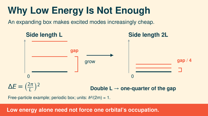
Energy estimates have long described dilute interacting Bose gases accurately. But low energy alone need not force a macroscopic population into one orbital in an expanding box.
For a free particle in these units, the first nonzero kinetic energy is . It approaches zero as the box grows. Consequently, an energy estimate can permit particles to occupy many increasingly cheap modes without providing a useful lower bound on constant-orbital occupation.
| Approach | Reach and Remaining Distinction |
|---|---|
| Ideal Bose gas | Noninteracting condensation does not establish condensation with an impenetrable core. |
| Bogoliubov expansion | Describes excitations around macroscopic occupation. Establishing that occupation for the exact state is a separate task. |
| Energy and free-energy bounds | Control thermodynamics, but alone need not force occupation into one mode as the kinetic gap closes. |
| Earlier GP condensation theorems | Establish condensation in specific scaling limits, including a vanishing scattering length in the homogeneous setting. |
| This hard-sphere theorem | Keeps exclusion distance, density, and positive temperature fixed before volume grows without bound. |
Earlier homogeneous positive-temperature GP results rigorously established condensation in their stated regime. Here GP abbreviates Gross–Pitaevskii. In that scaling, the scattering length decreases with system size. This manuscript instead fixes the physical hard core before taking the thermodynamic limit.
Effective wave models remain valuable. Our nonlinear Schrödinger equation guide explains their broader setting, but deriving properties of the exact many-body equilibrium state is a separate task. Likewise, a uniform spectral gap is a particular mathematical property, not a synonym for quantum coherence.
5. Turning a Thermal Mixed State Into an Overlap Problem
At positive temperature, equilibrium is a mixture of energy states. The canonical density operator is , where normalizes its trace.
The proof uses the nonnegative integral kernel of . Factoring the Gibbs operator through its square root turns occupation into an exact overlap. Abbreviate and , with . Then
Here contains the other particle positions, called the bath, and is an auxiliary retained configuration. Both factors must share exactly the same bath and retained data. Otherwise the comparison would concern a different quantity.
A short imaginary-time Brownian-path representation realizes as a probability density. Conditional on endpoints and retained data, the short paths are Brownian bridges conditioned to avoid hard-core collisions. Imaginary time is a representation of the equilibrium operator, not a filmed trajectory of atoms.
This conversion preserves off-diagonal information while giving the proof positive measures to compare.
The ground-state companion already developed the bridge-replacement and long-distance comparison mechanisms. This paper’s additional burden is thermal: establish the local conditions jointly under the interacting Gibbs path measure, then connect those comparisons to a mixed state’s one-particle density matrix. Both changes are needed. Carrying over a pure-state argument without rebuilding these links would leave the positive-temperature conclusion unsupported.
6. Controlling Particle Shortages and Excessive Crowding
The comparison needs cells containing enough well-separated particles. Two complementary estimates supply them. Confinement with hard exclusion costs kinetic energy, while inserting another particle can be done at controlled free-energy cost.
The insertion construction is normalized for each existing configuration. Integrating out the inserted particle therefore preserves the old position marginal. A uniform frame bound controls a family of insertion maps, allowing an entropy comparison rather than merely a trial-energy calculation.
Localization splits particles into auxiliary species through smooth position-dependent weights. This accounts for the kinetic price of localization and the entropy of the resulting states. Diagonal tilting reweights configurations so that free-energy inequalities can detect unusual local particle counts and excessive close neighbors.
These steps establish joint bounds: many prescribed cells simultaneously being deficient or poorly separated is exponentially unlikely. Independence is not assumed. That distinction matters because interacting particles correlate the regions being tested.
Entropy is therefore an active part of the positive-temperature argument. Readers familiar with our 2D area-law analysis will recognize the need to control reduced-state information carefully, although the entropies and conclusions here serve a different proof.
7. Controlling Whole Trajectories at Positive Temperature
Good endpoints do not guarantee good paths. A particle can begin and finish safely while making an inconvenient excursion between them. The proof must control complete trajectories during its short imaginary-time interval.
It marks paths failing regularity or confinement tests and assigns auxiliary species to those marks. Removing selected hard-core restrictions enlarges a path integral, providing an upper bound. This is a comparison device, not a change to the physical gas in the theorem.
A trace-sandwich estimate for heat evolution between Lipschitz multipliers converts marked-path moments into free-energy estimates. Exterior-power arguments extend the control to every positive trace power needed in the construction.
Combining endpoint and trajectory tests gives a certificate for usable cells. The resulting bounds remain joint bounds for arbitrarily many prescribed failures. If denotes the bad-cell set and any prescribed finite cell set, the eventual exposed environment satisfies
The parameter can be chosen sufficiently small.
8. Moving Particle Paths Without Violating the Hard Core
In a certified cell, many particle labels admit a short bridge replacement through a neighboring cell. Gaussian-density estimates and averaged collision bounds show that a substantial supply of these trials succeeds with uniformly positive probability.
The argument averages over candidate labels. It does not require every particle to be movable around every conceivable obstacle. That flexibility is essential when a particular local arrangement blocks one attempted move.
Useful labels are divided into disjoint groups. For one group, the proof exposes the surrounding paths and retains the appropriate endpoint and auxiliary data. The usable-cell environment then becomes determined by what has been exposed.
Conditioning is delicate. The remaining path law includes exact normalization factors for hard avoidance. Treating candidate bridges as independent after conditioning would discard those factors and break the later comparison.
The strategy has a thematic relative in positive-temperature Heisenberg ordering: local motion must ultimately support an infinite-volume order statement. Here, however, the particles move in continuum configuration space and the target is orbital occupation.
9. Connecting Distant Cells Around Sparse Obstacles
The proof now needs routes between distant usable cells. It constructs an auxiliary lattice of cells, draws randomized skeleton routes, and replaces portions crossing bad clusters with detours along suitable exterior boundaries.
This lattice organizes comparisons. It does not replace the continuum Hamiltonian with a lattice Bose gas. The distinction prevents a computational convenience from silently becoming a new physical assumption.
Ordinary connectivity is insufficient. Two independently sampled routes through the same exposed environment must also have controlled numbers of encounters, meaning pairs of nearby route vertices. The paper proves a bounded exponential encounter moment after the required environmental averaging, on an admissibility event of uniformly positive probability.
It does not promise a favorable bound in every fixed environment or for every pair of endpoints. Instead, a positive fraction of distant cell pairs supplies enough contributions for the final occupation average.
The geometry resembles questions introduced in our percolation theory guide, but the environment here is dependent and requires more than a connected crossing. The encounter estimate is tailored to the measure comparison that follows.
10. The Decisive Cancellation: Paying for Encounters Instead of Distance

A sequence of local moves can lose a fixed factor at each step. Multiplying those losses along an increasingly long route would produce a useless lower bound. The proof avoids that trap by comparing entire constructions after route averaging.
Along a route, it builds two midpoint assignments. Removing a different tagged particle from each leaves identical bath observations and the same retained configuration. These are exactly the matched variables required by the square-root overlap identity.
Conditional normalizers cancel away from encounters between two sampled route changes. The second-moment cost is therefore concentrated near mutual encounters, rather than growing with either route’s total length. The previous geometric estimate makes that remaining cost manageable.
The final measure inequality is elementary but powerful. If a common measure has mass and squared density integrals bounded by and relative to measures and , then
Affinity measures overlap. Disjoint tag groups and many distant cell pairs turn this positive overlap into a volume-uniform occupation bound. Connectivity alone would not have supplied that quantitative conclusion.
11. Returning to Physical Units and Identifying the Proof’s Limits
The scaled proof uses unit cells containing a large mean number of particles and a small scaled exclusion distance. Its parameters are selected in a prescribed order, all before volume tends to infinity.
Returning to physical units uses a length scale with a finite limit determined by fixed exclusion distance and density. The scaled temperature is . Choosing one positive physical temperature keeps the scaled system inside the proven range as the box grows. No volume-dependent cooling is hidden in the conclusion.
This is an existence theorem, not an optimized prediction of the transition temperature. It does not establish superfluidity, complete condensation, leading depletion, or improved performance for a sensor or quantum computer. For developers, the reusable idea is the comparison architecture, not a software speedup.
For researchers, the result supplies a precise foundation for asking sharper questions about temperature ranges and occupations. Those improvements need further estimates. In particular, a positive lower bound is compatible with a noncondensed population. Neither the constant orbital nor zero-momentum occupation implies that every particle is stationary, and the equilibrium system has one positive temperature.
The published Lean scope note covers the ground-state companion, explicitly without a positive-temperature assertion. Explaining this preprint is not an independent proof audit or a successful formal rebuild.
The Bose–Einstein condensation proof matters because its coherence bound survives an indefinitely growing sample. Follow Binary Verse AI for research explanations that track the model, the decisive argument, and the exact boundary of what has been established.
What does OpenAI’s Bose–Einstein condensation proof actually prove?
For the three-dimensional dilute hard-sphere gas, it establishes a positive limiting lower bound on the fraction occupying the constant orbital in the exact canonical Gibbs state at a strictly positive temperature. The exclusion distance, density, and temperature remain fixed while particle number and volume grow.
If Bose–Einstein condensates already exist experimentally, why was this proof needed?
Experiments establish condensation in physical systems. This mathematical problem asks whether condensation follows from a specified interacting many-particle model under a precise thermodynamic limit. Experimental observation and that mathematical derivation answer different questions.
Can Bose–Einstein condensation occur above absolute zero?
Yes. Positive temperature means above zero Kelvin, which can still be extremely cold. Condensation requires macroscopic occupation of one orbital. It does not require every particle to occupy that orbital or the equilibrium temperature to equal zero.
How can hard-sphere particles share one quantum state without overlapping?
The condensate orbital describes one-particle occupation. The full many-particle state also contains correlations enforcing hard-core exclusion. Macroscopic occupation of a constant orbital therefore does not mean the complete state is an uncorrelated product allowing particles to overlap.
How does this differ from ideal-gas, Bogoliubov, and Gross–Pitaevskii descriptions?
The ideal gas omits interactions. Bogoliubov theory expands around macroscopic occupation. Earlier Gross–Pitaevskii results rigorously establish condensation in particular scaling regimes. This paper addresses the exact hard-sphere equilibrium state while keeping exclusion distance, density, and positive temperature fixed as volume grows.
Does the proof determine the critical temperature or establish superfluidity?
No. It establishes condensation at a sufficiently low positive temperature without locating the phase-transition temperature. It also does not establish superfluidity, complete condensation, or the leading depletion formula.
Is the positive-temperature proof verified in Lean?
The listed Lean formalization concerns the companion ground-state condensation result. Its scope explicitly excludes a positive-temperature assertion, so it should not be presented as formal verification of this paper’s main theorem.