
A formula can give the right answer for twenty-two years without anyone knowing how to prove it. The Mezard Parisi formula faced precisely that problem: a hierarchy of cavity-field distributions supplied rigorous upper bounds for sparse spin systems, but the matching lower bound remained missing.
OpenAI’s September 23, 2026 paper proves that equality for the specified Panchenko–Talagrand class of diluted, even-arity Ising models. It resolves the variational conjecture stated in 2004 by controlling higher-order spin correlations and recovering independent hierarchical cavity messages. The result determines limiting pressure, hence physical free energy, under explicit assumptions. Its achievement is a rigorous bridge between the interacting system and the proposed trial formula.
Table of Contents
1. What Did OpenAI Prove About the Mezard Parisi Formula?
Theorem 2.1 in the original research paper establishes existence of the thermodynamic limit and identifies it exactly:
Here counts spins, is expected log partition function per spin, and is the optimized trial value at finite hierarchy depth . Taking the infimum permits arbitrarily deep finite hierarchies. It neither guarantees an optimizer nor constructs an infinite-depth Gibbs state.
| Research Detail | Verified Scope |
|---|---|
| Main result | Limiting expected pressure equals the infimum over finite hierarchy depths and trial laws. |
| Model class | Poisson-diluted Ising interactions of even arity, with factorization, independence and positivity assumptions. |
| Moment requirements | Finite first moments of the interaction supremum and absolute external field. |
| New ingredient | A matching lower bound obtained through finite-tree identities and multioverlap concentration. |
| Optimization scope | An infimum, without assuming attainment or constructing an infinite-depth Gibbs state. |
The paper calls pressure. With inverse temperature absorbed into the interactions and fields, physical free energy per spin is . Consequently, an upper pressure bound becomes a lower physical-free-energy bound. Keeping that sign straight prevents considerable confusion.
OpenAI released the mathematics collection on October 6. As our guide to AI mathematical proofs emphasizes, a manuscript, formalization documentation and independently reproduced verification are distinct evidence.
2. What Are Diluted Spin Glasses, and Why Is Their Free Energy Difficult to Calculate?
An Ising spin takes one of two values, plus or minus one. In a diluted model, each spin participates in a finite mean number of randomly placed interactions as system size grows. The local neighborhood remains random.
Frustration supplies the difficulty. Imagine three pairwise preferences around a triangle that cannot all be satisfied together. Sparse spin glasses contain competing constraints on a much larger scale, so their equilibrium behavior cannot generally be summarized by one favored configuration.
The partition function weights every configuration by its thermal contribution. Its logarithm balances energy against the number of available configurations. The thermodynamic limit asks whether this quantity per spin stabilizes as the system grows.
This differs from the alignment question in the quantum Heisenberg ferromagnet. Here the target is an exact variational pressure formula for classical random interactions, rather than spontaneous magnetization.
3. The 2004 Panchenko–Talagrand Conjecture: What Was Still Unproven?
Mézard and Parisi developed the hierarchical cavity picture for a fixed-connectivity Bethe-lattice spin glass. Franz and Leone adapted interpolation to diluted systems, obtaining replica-symmetric and one-step bounds. Panchenko and Talagrand extended the argument to arbitrary finite hierarchy levels.
Immediately after Theorem 4, their 2004 paper on diluted spin-glass bounds proposed that the optimized bounds were exact. The conjecture was about eliminating a possible gap between the true pressure and a particular hierarchical trial family.
Other exact variational descriptions existed, including formulations using spin distributions. An exact formula over a broader description does not automatically establish equality for this specific family.
Nor is this simply the classical Parisi formula again. The Sherrington–Kirkpatrick model has dense interactions. Sparse models require distributions of local cavity fields and more extensive replica information. Likewise, pressure is not the excitation-energy separation studied in the Laughlin spectral gap problem.
4. The Exact Mathematical Model: Poisson Interactions, Ising Spins, and Positivity
Fix an even arity and density . The interaction count is Poisson with mean . Each interaction samples its spin indices independently and uniformly, with replacement. Thus repeated indices are allowed.
Writing for the interaction evaluated at its sampled indices, the Hamiltonian convention is:
The partition function and pressure are:
The expectation averages the random interactions, fields, counts and indices. These families are mutually independent. The assumptions require , where .
Crucially, interactions must factor as , with and the absolute product term strictly below one. The functions are independent copies, independent of . Positivity means for every integer , with finite expectations. The multiplier may depend on the other factors. These conditions delimit the theorem’s reach.
5. How the Hierarchical Cavity Formula Works: Messages, Trial Laws, and Free Energy
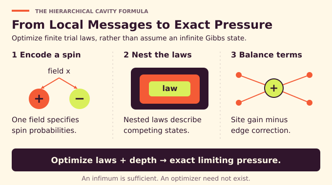
A cavity message is a real field encoding a one-spin probability law, . Large positive fields favor plus spins, while zero gives equal probabilities.
The site contribution inserts a new spin and its incident interactions, averaging neighboring spins against their message laws. The edge contribution corrects the interaction accounting. Without that subtraction, the site construction would count too much.
At depth zero, messages are independent draws from one probability distribution. At depth one, a label first draws a random probability distribution, then draws its field from it. Higher levels repeat this nesting of probability laws. This is how the trial class represents replica symmetry breaking: several competing statistical descriptions survive instead of one common field law.
Parameters govern backward conditional power means:
Here records the physical disorder and message information through level . Only auxiliary descendants are averaged, with physical disorder fixed. The trial functional is:
The symbols and denote site and edge factors, while specifies the nested trial law. Optimize over and the exponent vector to obtain . The theorem then optimizes over depths. It does not prescribe one numerical hierarchy that solves every instance.
The new site receives a Poisson number of interactions with mean . Its spin is summed over both signs, with a factor of one half in . The separate restores that normalization. These constants are part of the identity, not optional conventions.
6. Why the Previous Interpolation Method Could Prove Only the Upper Bound
Interpolation gradually replaces genuine interactions by independent cavity interactions. At one endpoint lies the interacting system. At the other, site contributions factor through the hierarchy.
The derivative contains a convexity remainder. Schematically, for real comparison quantities and , even arity gives:
Together with the positivity moments, this fixes the derivative’s sign and proves for every system size and trial law.
That direction is powerful but insufficient. A family of upper bounds could remain strictly above the true answer, regardless of how cleverly it is optimized. Establishing equality requires finding admissible hierarchical laws whose values approach the actual pressure from the other side.
OpenAI’s proof therefore needs a reconstruction argument. It must extract the right trial messages from a real interacting system while controlling the error caused by making them independent.
7. The Hidden Obstacle: Why Pair Overlaps Cannot Determine All Replica Patterns
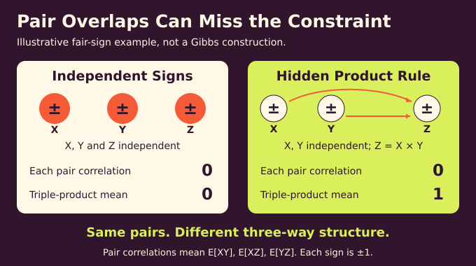
Replicas are repeated samples from the same Gibbs system, not additional physical copies wired together. A pair overlap averages the product of two sampled spins across sites. For any subset of replica labels, the multioverlap is:
Pair information misses higher-order structure. Take two independent fair signs and define a third as their product. Every pair has zero correlation, yet the product of all three is always one. Three independent fair signs have the same pair correlations but triple-product expectation zero.
This example is explanatory, rather than a claimed Gibbs construction. It shows why reconstructing joint replica patterns from pairs alone fails.
For Ising variables, the empirical probability of each complete replica-spin pattern expands in products indexed by every replica subset. All finite multioverlaps therefore matter. Independent message labels reproduce the cavity insertion only after this richer pattern information is controlled. Sparse systems leave no room to discard it merely because pair overlaps look well behaved.
8. OpenAI’s First Breakthrough: Finite-Tree Insertion Calculus and the Cavity Reservoir
OpenAI’s proof starts with finite auxiliary probability trees. A root stores disorder. Paths successively sample auxiliary variables and finally a Gibbs configuration. Shared prefixes and independent descendant branches encode prescribed replica relationships.
These trees are bookkeeping devices constructed for the argument. Their shape is not an assumed description of physical Gibbs states.
The insertion calculus tracks how multiplying the terminal weight by an extra factor changes backward power means. Differentiation produces signed combinations of added replica paths. A logarithmic expansion then expresses insertion free energies through averages over finite trees.
Next comes the reservoir: one common system used to compare sizes and . Adding a spin produces a site insertion, while correcting the old interactions produces a bond subtraction.
Bounded perturbation factors arrive in a Poisson number with mean . Their total contribution per spin vanishes. Nevertheless, their derivatives supply useful identities. The proof selects system sizes and deterministic perturbation parameters that simultaneously control these scores and keep the cavity increment close to the original pressure’s lower limit.
That simultaneous selection matters. Convenient identities alone would be useless if obtaining them moved the comparison away from the thermodynamic quantity being proved.
9. How Perturbations Recover Prescribed Replica Branching Patterns
A perturbation score measures sensitivity to its parameter. At fixed finite depth, concentration makes the normalized score’s fluctuations vanish along the selected sequence. Insertion expansions convert this concentration into identities for replica observables.
Independent signs, or marks, are sampled at selected tree depths. Two replicas sharing a vertex share its mark. Separate vertices receive independent marks. Products of colored marks can therefore select particular splitting patterns, allowing the argument to target a prescribed finite replica tree.
The resulting identities involve signed extension coefficients. Some coefficients become small as depth increases. Dividing by them without tracking errors would risk amplifying a harmless approximation into a fatal one.
The remedy is to delay each internal target split by one level. A newly required branch must then split at a previously unbranched vertex. Each such fresh split contributes the same small factor needed by the normalization. A relative bound controls the total absolute coefficient cost after division.
The order of limits is essential: system size goes to infinity at fixed depth before depth increases. Errors in fixed-tree identities disappear before small denominators become a problem. The paper does not require a convergence rate uniform in hierarchy depth.
10. Concentrating Multioverlaps and Recovering Independent Cavity Messages
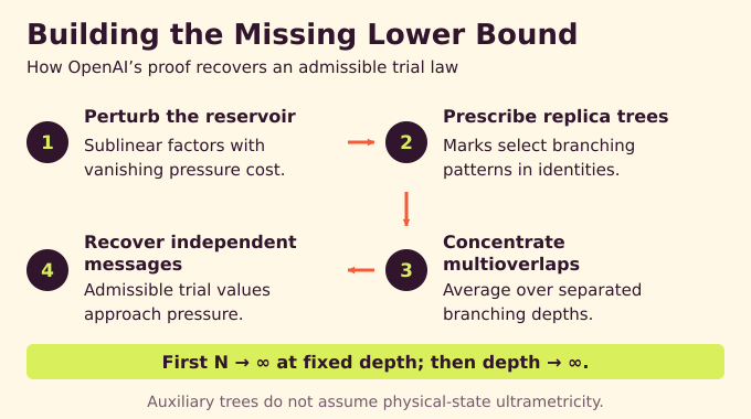
The decorrelation argument proceeds by induction on replica number. It first controls conditional covariances of spin-product vectors below a sampled prefix. Proper child trees contain fewer replicas, so their contributions can be replaced by conditional means using the induction hypothesis.
Prescribed-tree identities compare delayed copies of the target tree. After the signed terms are combined, they produce nonnegative estimates that force the relevant covariance averages down. A second identity, using a marker anchor, concentrates the remaining conditional mean.
The result is multioverlap concentration averaged over separated interior branching depths. Uniform control of every tree is unnecessary: exceptional branching assignments have vanishing weight in the logarithmic insertion expansion.
Finally, choose a uniformly random reservoir site. Its conditional spin mean defines a field, . Successive conditional laws encode that site’s entire finite hierarchy as an admissible trial law. Different labels receive independent copies.
Multioverlap concentration ensures that this replacement preserves the needed replica-pattern averages, hence the insertion logarithms after controlled cutoffs. The site-minus-bond increment becomes a genuine hierarchical trial value.
The comparison first cuts off large Poisson interaction counts, then truncates the logarithmic series. Only finitely many replica patterns remain to check. Their errors vanish in the ordered limits, after which the count and series tails are removed using explicit bounds.
This supplies the missing bridge. Auxiliary branching is imposed by construction, while physical Gibbs-state ultrametricity is never assumed. The proof recovers the variational answer without first classifying every equilibrium state.
Independence here concerns replacement labels inside this comparison. It does not say that every pair of physical spins becomes independent, or that frustrated interactions disappear. Their thermodynamic effect remains encoded in the nested law and the site and edge terms.
11. Closing the Proof: The Matching Lower Bound, Model Applications, and Mathematical Limits
For bounded, permutation-invariant interactions, the reconstructed trial values establish the lower bound. Factorization and positivity are needed for the upper bound, rather than this bounded-law lower-bound argument.
To finish, subtract the integrable constant . This removes the potentially asymmetric multiplier and makes the normalized interaction law permutation invariant. Truncate interactions and fields, apply the bounded result, then remove the cutoff. Stability estimates uniform over trial laws and depths make first moments sufficient.
Importantly, this route does not assume separate integrability of . The subtracted constant is bounded in absolute value by , whose expectation is already finite. Both pressure and the trial functional shift by the same amount.
| Model | Application and Qualification |
|---|---|
| Viana–Bray | Two-spin case with symmetric integrable couplings and integrable fields. |
| Diluted even-spin models | Even interaction arity with symmetric integrable couplings, at every positive temperature. |
| Soft random even- SAT | Even clauses with independent fair literal signs and independent nonnegative integrable weights. |
| Random 3-SAT | Excluded by this theorem’s even-arity assumption. The paper identifies a different companion formulation. |
For these named models, pressure divided by lies above the limiting expected maximum score per spin by at most . The score is the temperature-independent quantity multiplied by in the Boltzmann exponent. Cooling therefore yields the zero-temperature variational limit. For unit-weight SAT, negating that score yields the limiting expected minimum violations per variable.
This is an asymptotic characterization, not a practical solver benchmark. Unlike an algorithmic result such as the subset sum runtime improvement, it supplies no demonstrated speedup for finding configurations. Nor does it settle approximation hardness questions of the kind discussed in our Unique Games explainer.
OpenAI’s paper-specific Lean scope note describes a formalization of the main equality under its assumptions. This article does not report an independent Lean rebuild or establish journal peer-review status.
The Mezard Parisi formula now has the matching argument its trial bounds required: control complete replica patterns, recover independent messages, and close the variational gap. Follow Binary Verse AI for further research explainers that unpack the mechanism and keep the theorem’s boundaries visible.
What is the Mézard–Parisi formula?
It is a hierarchical cavity variational formula for the limiting pressure, and consequently the physical free energy, of certain diluted spin-glass models. OpenAI’s proof establishes its exactness for the specified Panchenko–Talagrand class.
What was the Panchenko–Talagrand conjecture?
The 2004 conjecture asked whether the finite-level hierarchical variational upper bounds were sharp after optimization over all finite depths and trial laws. OpenAI’s proof establishes the matching lower bound, turning the inequality into equality.
How is the Mézard–Parisi formula different from the classical Parisi formula?
The classical Parisi formula describes densely connected mean-field spin glasses, particularly the Sherrington–Kirkpatrick model. The result studied here concerns sparse random interactions and hierarchical distributions of cavity fields.
What does the cavity method mean in spin-glass mathematics?
The cavity method studies how adding a spin and its interactions changes the system’s partition function. Its hierarchical version uses nested distributions of cavity messages to describe multiple competing thermodynamic states.
Why are multioverlaps essential to OpenAI’s proof?
Pair overlaps alone do not determine joint spin patterns across several replicas. Controlling all finite higher-order multioverlaps permits the replacement of dependent reservoir-site patterns by independent hierarchical message patterns in the cavity comparison.
Does the proof apply to every spin glass and random SAT problem?
No. The theorem applies to the specified Poisson-diluted even-arity Ising class satisfying factorization, independence, positivity and integrability assumptions. It includes Viana–Bray and soft random even- SAT, but excludes random 3-SAT under this theorem.
Does OpenAI’s proof determine spin-glass ground-state energies?
Section 10 establishes a zero-temperature variational limit for the named spin and soft even-clause SAT models. It characterizes the limiting expected optimum per spin or variable, but does not compute an explicit optimal configuration for every finite system.