
A magnet should not need a mathematical permission slip to stay magnetized. Yet proving positive-temperature order in the quantum Heisenberg ferromagnet required much more than showing that neighboring spins prefer alignment.
OpenAI’s September 24, 2026 paper supplies that proof for the nearest-neighbor isotropic model on the integer lattice in every dimension , for every positive integer or half-integer spin. At sufficiently low positive temperature, it constructs a translation-invariant equilibrium state for the zero-field dynamics with magnetization at least . The achievement is an ordered infinite-volume state, rather than an exact Curie temperature or a simulation of a commercial magnet.
The central advance is a chain of reductions: interacting spins become exchange loops, boundary pins become return estimates, and diffusion estimates ultimately yield a genuine equilibrium state.
Table of Contents
1. What OpenAI’s Quantum Heisenberg Ferromagnet Proof Establishes
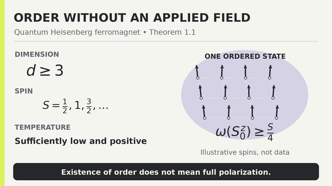
Theorem 1.1 in the research paper fixes a dimension and spin, then establishes a finite inverse-temperature threshold . Every finite at or above that threshold admits a translation-invariant state satisfying the Kubo–Martin–Schwinger, or KMS, equilibrium condition and
Here is the spin’s vertical component at the origin, and gives its expectation. Translation invariance makes the same expectation hold everywhere. For , the guaranteed magnetization is . The bound is positive and uniform across lattice sites, without asserting saturation.
| Feature | Proved Scope |
|---|---|
| Interaction | Nearest-neighbor isotropic exchange, coupling one |
| Lattice And Spin | Integer lattice, ; |
| Temperature | Sufficiently low and strictly positive |
| State | Translation-invariant KMS state for zero-field dynamics |
| Order Parameter | One-site magnetization at least |
OpenAI’s mathematics release announcement places the work within results produced by an internal frontier model. Readers following AI mathematical proofs should distinguish that provenance from what this particular theorem establishes.
2. The Original Problem: Can Quantum Spins Align Without An External Magnetic Field?
The model assigns a spin space to each site of a finite region . Its exchange Hamiltonian is
The vector contains operators, rather than classical arrows. The sum counts each unordered neighboring pair once. Its negative sign favors parallel alignment, while treating all spin directions equally. Coupling is normalized to one, so the paper’s temperature threshold is expressed in those mathematical units.
A fully aligned lowest-energy state does not settle the thermal problem. At positive temperature, excitations can reduce magnetization, and long-wavelength fluctuations can accumulate as the system grows. The question is whether some directional preference survives those fluctuations throughout an infinite lattice.
Inverse temperature obeys in physical units. Thus large inverse temperature means low temperature. Crucially, the theorem keeps that temperature positive while taking the system size to infinity. Cooling a finite system all the way to its ground state would answer a different question.
3. Why Proving Spontaneous Magnetization In Three Dimensions Was So Difficult
A finite zero-field Gibbs state inherits rotational symmetry. Its average spin therefore vanishes. Infinite systems allow a different possibility: individual equilibrium states can choose directions even though their rotation-invariant mixture has no preferred direction.
Imagine averaging equally over magnets pointing in every direction. The ensemble has zero mean magnetization, but that cancellation does not erase the ordered states used to construct it. Quantum ferromagnet spontaneous symmetry breaking concerns those individual states. Zero expectation in the symmetric average is not a disproof.
Dimension matters because fluctuations behave differently across scales. Mermin–Wagner excludes the corresponding positive-temperature ferromagnetic order in the finite-range isotropic model in one and two dimensions. A 3D Heisenberg ferromagnet escapes that obstruction, but escaping a prohibition is not an existence proof.
The assumptions deserve the same attention as in the Haldane gap problem: changing dimension, interaction, or spin can change the mathematical question. Here the proof must control arbitrarily large distances at one fixed positive temperature.
4. The Decades-Old Barrier: Why Earlier Mathematical Methods Failed
Lieb explicitly posed the quantum ferromagnetic ordering problem in 1999. Established infrared-bound methods had proved major classical ordering results and quantum antiferromagnetic results. Their reflection-positivity argument did not yield the ferromagnetic Duhamel infrared bound needed here. The useful estimate failed to transfer between models.
An infrared bound controls low-frequency fluctuations, precisely where large-scale disorder can hide. Without the appropriate bound, the intuition that three-dimensional spins should remain aligned did not complete the argument.
Spin-wave theory offered another important success. Rigorous work established fixed-spin low-temperature free-energy asymptotics in three dimensions, with correlation estimates on a temperature-dependent finite length scale. Those results did not construct the magnetized equilibrium state required at arbitrarily large distances.
This distinction also matters when reading about the Laughlin spectral gap or a two-dimensional area law. Controlling an energy quantity, a gap, an entropy bound, and an ordered thermal state are distinct accomplishments. OpenAI’s proof addresses the missing state construction through a probabilistic route.
5. OpenAI’s New Proof Begins With Spin Slots, Exchange Loops, And Boundary Pins
First replace each spin by spin-half slots and restrict them to their symmetric subspace. This reproduces the original spin representation exactly. It is not an approximation that weakens quantum interactions into classical ones.
Each neighboring slot pair exchanges along a rate-one-half Poisson clock over a time period of length . Uniform permutations within each site connect the period’s endpoints. Following the resulting lines produces cycles that may wind through several periods.
This time coordinate belongs to the Gibbs representation, rather than the physical dynamics checked at the end.
Every cycle receives a weight of two because it has two possible spin colors. Coloring cycles then reproduces the full spectral distribution of total magnetization, not merely its mean. That stronger identity becomes essential when a field selects a magnetization tail later.
A pin requires its entire cycle to have the up color, reducing that cycle’s weight from two to one. Pinning every boundary slot throughout the period creates a directional reference. Positive weights alone were already available in earlier representations. The missing ingredient is a uniform estimate showing that an interior cycle rarely avoids this pinned boundary.
6. How Stable Polynomials And Negative Dependence Control The Loops
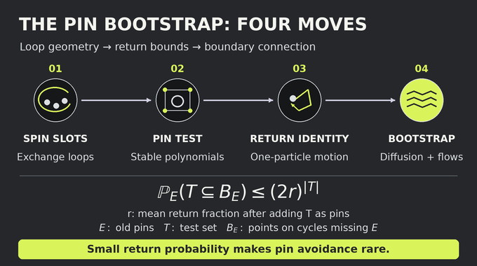
Let denote existing pins, a set of test points at one time, and the points on cycles avoiding . Add the test points as pins, giving . Under this larger-pin law, is the average fraction of test lines that return to the test set at positive elapsed time before reaching an old pin.
Proposition 3.1 proves the simultaneous pin test:
This converts a potentially troublesome joint avoidance event into a mean return estimate. The factor two comes from comparing the two pin laws. It is not an assumption that individual loop events are independent.
The algebra uses stable multiaffine polynomials: each variable has degree at most one, and the polynomial has no zero when all variables have positive imaginary parts. Stability survives carefully chosen exchange and elimination operations. The resulting strongly Rayleigh-type negative dependence bounds simultaneous presence by products of individual presence probabilities.
The relevant random subset consists of outputs of the next-pin permutation. If every test point’s cycle misses the old pins, the next-pin map sends the test set onto itself. Stability bounds this whole-set event through the individual output probabilities. Their arithmetic mean is exactly the return fraction, which produces the power appearing in the pin test.
For the later bootstrap, test sets satisfy a sparse spatial-growth condition. This restriction still includes a single interior slot and the separated witnesses needed to detect large obstacles. The proof does not require unrestricted independence across the lattice.
7. Turning An Interacting Quantum Problem Into A One-Particle Return Identity
Next expose exactly the cycles avoiding the enlarged pin set. The remaining slots, called holes in the proof, carry a conditional exchange process in which every remaining cycle must meet a pin. That conditioning creates dependencies, so simply replacing the picture by independent random walks would be unjustified.
The escape route is a determinant identity. Before all-hit conditioning, the relevant random permutation matrix satisfies
The exterior power records all minors of a given size . Independent Bernoulli transpositions have the required determinant-preserving property, which survives independent products and the exchange-process limit.
A further calculation recovers every entry of the conditional next-pin first moment as the hitting kernel of one Markov walker using fresh randomness on successive steps. Every entry matters: returning to another test point counts, not just returning to the starting point.
The matrix calculation separates pinned and unpinned coordinates. Its inverse term sums paths spending successively longer times among unpinned coordinates before hitting a pin. A determinant gives the probability of the all-hit conditioning event. Dividing by that probability produces the conditional first moment without discarding the conditioning.
This identifies a specific first moment, not the full conditioned process with independent walks. The exposed environment retains its original weighted marginal. Keeping that distinction intact is what makes the reduction useful rather than wishful.
8. Sparse Obstacles, The Nash Inequality, And Diffusion Around Blocked Spins
A site is blocked when none of its slots remains available after exposure. The induction hypothesis controls simultaneous blocking for prescribed sparse collections. From these estimates, the proof builds separated witnesses that force large blocked components to contain many unlikely blocked sites.
The resulting component tails limit how large obstacles become. Near regular anchors, sufficiently few local deletions preserve short connections between surviving sites. Those connections transfer a lattice Nash inequality to the available-slot graph.
A Nash inequality links mass, squared concentration, and Dirichlet energy. In practical terms, concentrated probability must spread or pay an energy cost. Here that principle survives the changing geometry and boundary killing of the exposed process.
Farther away, the proof routes decaying finite-energy flows around blocked components. These flows control overlap terms that local spreading alone cannot handle. The geometric viewpoint connects naturally with nonamenable percolation and probabilistic connectivity proofs, although the obstacles here come from conditioned spin loops rather than independent site deletion.
The flow construction starts from transient-lattice geometry available in dimensions at least three, then repairs routes around filled obstacle hulls. Both local and distant controls are necessary. Nearby connectivity prevents immediate trapping, while the global energy comparison prevents distant obstructions from ruining the return estimate. Sparse test growth also keeps overlaps between different starting-point flows summable.
9. The Heat-Flow Bootstrap That Closes OpenAI’s Proof
Let and let be the one-period walk kernel with killing at the boundary. Define to equal one on the test set and, elsewhere, the probability of eventually hitting it before killing. The required estimates combine as
The error satisfies : relative to , it vanishes as decreases. Consequently the return fraction becomes small enough to recover the desired avoidance bound.
The middle expression averages over exposed environments, and the quadratic form measures one-period loss. The difficult term appears after splitting , with the indicator equal to one exactly on the test set. Although the two pieces initially have disjoint support, their propagated masses can overlap. Local Nash diffusion spreads the test mass, while the routed flows bound its pairing with the other part through energy measured at the same time.
Weighted time averaging absorbs that pairing into heat dissipation. Choosing small enough that makes the pin test give . Downward induction starts with all grid points pinned, then removes pins. Because the grid is finite, this is a closing induction, not circular reasoning.
At the end, only continuous boundary pins remain. A single interior slot is unlikely to lie on a cycle missing them, uniformly in the box size.
| Bottleneck | Mathematical Tool | What It Supplies |
|---|---|---|
| Joint Cycle Avoidance | Stable-polynomial pin test | A bound through the mean return fraction |
| Conditioned Exchanges | Exterior-power identity | The full next-pin first-moment matrix |
| Irregular Available Geometry | Local Nash inequality and routed flows | Diffusion and overlap control |
| Boundary-Selected Order | Spectral tail and vanishing field | A magnetized state for zero-field dynamics |
10. From Pinned Loops To A Magnetized Zero-Field KMS Equilibrium State
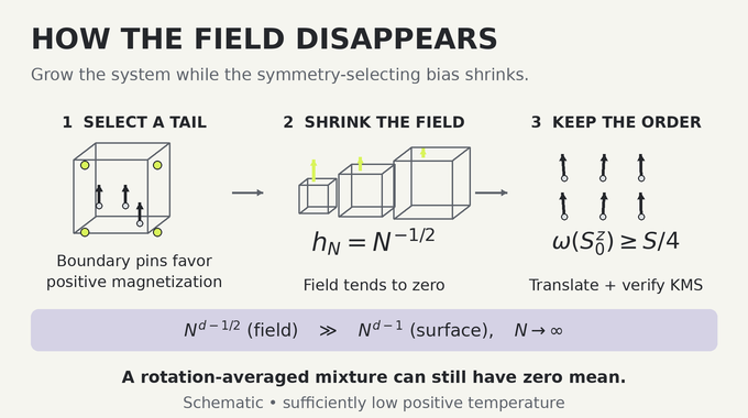
Boundary alignment is a tool, not the final Hamiltonian. Requiring every boundary-touching cycle to be up has a probability whose logarithmic cost scales with boundary size. The spectral representation transfers this into a tail of the free zero-field Gibbs distribution, with total magnetization at least .
A homogeneous field selects that tail in boxes of radius . Its bulk contribution grows like , faster than the surface cost , even though the field itself tends to zero. Translation averaging and subsequence extraction then produce the magnetized infinite-volume state.
The last step checks thermal equilibrium for the original zero-field dynamics. For observables and , the KMS condition requires a bounded function, continuous on the closed strip and analytic inside, with both boundary identities:
Here denotes zero-field time evolution, is real, and the strip has height in the imaginary-time direction. Reversing the operator order on its upper boundary encodes thermal equilibrium.
The proof controls dynamics far from translated box boundaries and passes both identities along the same state subsequence. Norm approximation extends the local-observable conclusion to the full algebra. A positive magnetization limit alone would not establish this equilibrium condition.
The ordering of limits matters. Sending the field to zero in each finite box would restore rotational symmetry before the infinite system could select a direction. Here the growing volume amplifies a shrinking field, and the eventual dynamics still has no field. Translation averaging removes dependence on the observation site while preserving the directional magnetization.
11. What The Quantum Heisenberg Ferromagnet Proof Settles And What Remains Open
The quantum Heisenberg ferromagnet proof establishes positive-temperature spontaneous magnetization for every allowed spin in dimensions at least three. The bound certifies order. It neither predicts exact magnetization nor calculates an exact Curie temperature, and the paper distinguishes its one-point state theorem from the separate finite-volume two-point ordering criterion.
For spin one-half, the correspondence also yields averaged off-diagonal long-range order in an attractive hard-core hopping model. After rotating the ordered state, the averaged correlation has a lower bound of . This concerns restrictions of the chosen infinite-volume state, not finite-volume Gibbs states or measured device performance.
The Lean scope note describes the magnetization theorem and dynamics convergence. A separate Lean solution file contains the theorem proof. The comparator’s sorry is a challenge placeholder, not evidence that this solution is incomplete. Binary Verse AI has not independently compiled or audited the complete formalization, a distinction also relevant to reading Lean proof coverage.
The useful takeaway is the bridge from loop control to zero-field equilibrium. Follow Binary Verse AI for research explainers that trace that bridge, check its assumptions, and make the mathematics readable.
What is the quantum Heisenberg ferromagnet?
It is a quantum spin model in which neighboring lattice spins interact through an isotropic exchange Hamiltonian favoring parallel alignment. OpenAI’s paper studies spontaneous magnetization at positive temperature in equilibrium states for the model without an applied magnetic field.
What exactly did OpenAI prove about spontaneous magnetization?
For every dimension of at least three and every positive integer or half-integer spin , OpenAI’s proof establishes a translation-invariant KMS equilibrium state for the zero-field dynamics with magnetization at least at every sufficiently low positive temperature.
Why does the proof apply to three dimensions but not one or two?
The Mermin–Wagner theorem excludes the corresponding positive-temperature ferromagnetic order for the finite-range isotropic model in one and two dimensions. The new proof establishes the ordered-state result for every dimension of at least three.
Why couldn’t previous mathematical methods prove low-temperature ferromagnetic order?
Reflection-positivity methods proved important classical and quantum antiferromagnetic ordering results but did not supply the required ferromagnetic Duhamel infrared bound. Later spin-wave results controlled free energy and correlations on finite temperature-dependent length scales without constructing the magnetized equilibrium state established here.
How does OpenAI’s new proof overcome the mathematical barrier?
It represents quantum spins through exchange loops, uses boundary pins and stable polynomials to control simultaneous avoidance events, and identifies the relevant return first moment with one-particle motion. Diffusion estimates, finite-energy flows, and a heat-flow bootstrap then support the construction of a magnetized zero-field equilibrium state.
How can spontaneous magnetization exist without an external magnetic field?
The Hamiltonian remains rotationally symmetric, but an infinite-volume equilibrium state can select a spin direction. The proof constructs such a state by taking growing boxes with a magnetic field tending to zero, then verifies equilibrium for the zero-field dynamics. Averaging the ordered state over all rotations can cancel its magnetization.
Does OpenAI’s proof determine the exact Curie temperature or prove every formulation of long-range order?
No. It establishes ordered equilibrium states below a sufficiently low positive temperature threshold without determining the exact critical temperature. Its main theorem concerns magnetization in a chosen infinite-volume state, rather than the separate finite-volume two-point correlation criterion.