

A particle can ricochet inside a triangle forever, obeying one elementary reflection rule, while hiding a difficult question: does its motion explore position and direction in the correct statistical proportions? OpenAI’s September 25, 2026 manuscript presents a proof that irrational triangular billiards are ergodic whenever at least one interior angle is an irrational multiple of π. It requires no special rational-approximation condition.
The advance concerns triangular billiards ergodicity for arbitrary measurable invariant sets, including sets whose boundaries offer no convenient smoothness. Below, we follow that argument, separate its classical and quantum conclusions, and examine why the public Lean evidence needs a qualification. This belongs to the same careful reading of AI mathematical proofs that asks what each artifact actually establishes.
Table of Contents
1. What Are Irrational Triangular Billiards, and Why Was Ergodicity Unsolved?
The table is an ideal Euclidean triangle. A point particle moves at unit speed and reflects specularly: the velocity component parallel to a side stays unchanged, while the perpendicular component reverses. There is no friction, rounded corner, or probabilistic bounce.
“Irrational” describes the table’s angles, not the starting direction. If an interior angle has irrational ratio , the triangle qualifies. Since its three angles sum to , exactly one irrational ratio is impossible. There must be two or three.
| Feature | Scope |
|---|---|
| Research document | OpenAI preprint dated September 25, 2026 |
| Eligible tables | Every nondegenerate Euclidean triangle with an irrational angle ratio |
| Invariant measure | Normalized area times uniform direction |
| Classical conclusion | Every measurable invariant set has probability zero or one |
| Excluded trajectories | Vertex hits in either time direction, a measure-zero set |
| Quantitative guarantee | No convergence rate supplied |
Ergodicity rules out a hidden compartment of positive probability that trajectories cannot leave. Its time-average interpretation holds for almost every initial state. A picture that fills the triangle can still miss the issue, because a state includes direction as well as location. Straight sides provide no dispersing curvature to make a familiar chaotic-billiards argument available.
2. What Exactly Does OpenAI’s Ergodicity Theorem Prove?
Theorem 1 in the September ergodicity manuscript concerns the full phase space . Here is the triangle’s interior and is the circle of unit velocity directions. Its probability measure is:
The numerator combines area and angular elements. The denominator normalizes the whole phase space to probability one. Writing for evolution through time, the billiard flow ergodicity conclusion is:
The triangle symbol denotes symmetric difference: membership differs between the two sets. Thus invariance is understood up to measure zero, for every time. Applying the criterion to a set’s indicator function reduces the task to proving that bounded invariant functions are constant almost everywhere.
Vertex hits have no prescribed continuation, so they are discarded. Their initial states form a null set. This qualification does not mean every remaining orbit is individually typical, or that every invariant probability measure equals the displayed measure.
For example, asking whether time spent in a chosen region matches its area is only a positional test. One can also select a region together with a range of velocities. Ergodicity controls such joint observables through almost-everywhere time averages, without promising a particular finite sampling duration.
3. The Decades-Old Barrier: Why Earlier Mathematical Proofs Fell Short
Zemlyakov and Katok established the unfolding connection between polygonal billiards and flat geometry. For rational polygons, the finite reflection group leaves invariant directional surfaces. Kerckhoff, Masur, and Smillie proved unique ergodicity in almost every direction on the associated surfaces, and obtained full-flow ergodicity for a dense countable intersection of open families of tables.
That distinction anchors rational vs irrational triangular billiards: good behavior within a directional surface does not make the full rational phase space ergodic. Nor does a generic-family theorem settle every irrational triangle.
Vorobets supplied explicit ergodic examples under exceptionally strong simultaneous rational approximation of angles. Chaika and Forni later proved weak mixing for a dense countable intersection of open sets of polygons with any fixed number of sides at least three. Again, genericity leaves individual tables uncovered.
The Forni–Moll analytic framework isolates another barrier. Constancy of geodesic-invariant functions follows with a suitable horizontal Sobolev assumption, . An arbitrary bounded invariant indicator need not have those square-integrable derivatives. Assuming them would assume away the problem. Ergodic billiards required a way across that regularity gap.
4. Unfolding the Triangle: How Reflected Paths Become Straight Geodesics
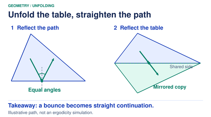
Instead of bouncing a path at an edge, reflect the triangle and continue the path straight. The paper packages this idea into a flat double: glue two copies with opposite orientations along corresponding sides. Remove the three vertices. The resulting connected surface is regular across open edges, while its completion has cone angles .
Geodesic motion on its unit tangent bundle folds back to the original billiard. The two equally weighted sheets reproduce the normalized area-and-direction measure. Chart changes involve rotations and translations, so local straight-line calculus remains available.
For each finite sequence of crossed sides, hitting a vertex becomes the condition that an unfolded straight line passes through a fixed point. That has measure zero. Countably many side sequences still give a null union. The paper also excludes a hidden failure mode: infinitely many reflections cannot accumulate in finite time away from the already excluded vertex hits.
5. Angular Fourier Modes: Turning Ergodicity Into a Transport Equation
Take a bounded invariant function upstairs. Let differentiate along a geodesic and in the perpendicular, parallel-transported direction. Invariance gives in the distributional sense, meaning after testing against smooth functions supported away from the cone points.
Decompose the directional dependence into angular harmonics . Each coefficient records one angular frequency. Because charts rotate, these coefficients are sections of flat unitary line bundles, rather than ordinary globally defined scalar functions.
The Cauchy–Riemann operators and combine the two spatial derivatives. The transport equation becomes:
This couples coefficients two indices apart. Even and odd chains can therefore be treated separately. The triangular billiards proof must first show every coefficient has an spatial gradient, then show each gradient vanishes. Those are different achievements. A bound for every individual mode does not imply the sum of all their squared gradient norms is finite.
6. The First Breakthrough: Controlling Singularities Without Assuming Smoothness
The manuscript smooths in position only, using a radial convolution kernel inside safe flat disks. It then multiplies by a cutoff that vanishes near each cone tip. The resulting field has compact spatial support in the regular surface, so integration by parts creates no unexamined corner term.
Lemma 3 supplies the localized estimate:
Here labels a Fourier coefficient, is the flat spatial gradient, and the subscript 2 denotes the square-integrable norm. The indicator restricts the final gradient norm to , the base region outside which applied to vanishes. The hypotheses also require both horizontal derivatives of to be square-integrable.
The mechanism is a telescoping energy identity along a parity chain. Integration by parts equates the two Cauchy–Riemann derivative norms. The mode recurrence compares successive energies. Cauchy–Schwarz then bounds their telescoped sum using only the region where transport invariance fails.
For a bounded locally invariant function with bound , that failure occurs in cutoff annuli of area . Derivative sizes are . Squaring and integrating over the shrinking annuli gives bounded norms, rather than a divergence. The estimate yields , uniformly in the Fourier index and smoothing scale, with a constant depending on the fixed triangle.
It supplies individual weak derivatives without asserting their square summability across modes. As with the assumptions in the Navier–Stokes proof analysis, the exact function space determines which argument is legitimate.
7. How OpenAI’s Proof Uses Long Trajectories to Eliminate Fourier Derivatives
Fix an index m and collect the modes starting there in steps of two. If the projection onto mode k is denoted by P with subscript k, the endpoint identity is:
Neighboring terms cancel through the recurrence. A finite tail has another endpoint at high angular frequency. Its norm need not vanish. Instead, its pairing with any fixed square-integrable test field vanishes as that frequency escapes to infinity. This is weak convergence, sufficient for the identity.
The next construction uses trajectories staying at least a fixed multiple of from every cone for time , where is fixed and positive. A time mesh and the quadratic area of cone neighborhoods bound the discarded probability by a constant times s plus the square of the smoothing scale.
Average the invariant function, restricted to these good starting states, backward over that interval. The resulting remains bounded, vanishes near the cones, approximates , and has transport derivative bounded by twice the function bound divided by . Differentiating this average produces an endpoint difference, without differentiating the rough good-set indicator.
Integrating the smoothed endpoint equation along good segments turns it into endpoint terms divided by the long flight time. A scaled smoothing-derivative estimate makes the resulting pairing tend to zero. This uses controlled clearance and averaging, not an assumption that trajectories mix rapidly.
8. Why Two Successive Limits Complete the Most Difficult Step
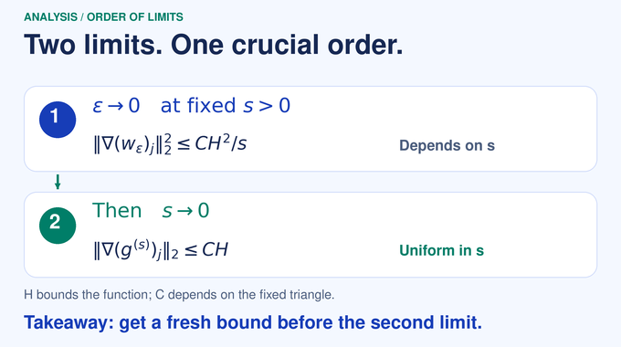
First send the smoothing scale to zero while keeping fixed. Smoothed averages have a weak limit solving the exact local transport equation. Their distance from is bounded by . Bounds for the relevant coefficient gradients let the vanishing endpoint pairing survive this passage.
However, the squared-gradient bound available at this stage grows like . It deteriorates as shrinks. Sending both parameters to zero together would leave the crucial derivative limit uncontrolled.
The repair is to apply the bounded-coefficient estimate again to . This is now legitimate because the first limit produced an exact local equation and retained the original uniform bound on the function. The new gradient estimate is independent of .
The first passage needs only a fixed pair of coefficient derivatives, not the full transverse derivative of the weak limit. Projection onto the endpoint mode selects exactly those terms. This prevents an unjustified global Sobolev assumption from slipping back into the argument during the compactness step. Uniform boundedness of the limiting function is what makes the second application possible.
Only then send to zero. The functions converge strongly to , while the relevant gradients converge weakly with uniform bounds. The pairing passes to the limit. Since the recurrence gives , its vanishing forces to be zero. Repeating for every endpoint eliminates every coefficient gradient. The order of limits is part of the proof, not a cosmetic choice.
9. Why One Irrational Angle Forces the Final Ergodicity Conclusion
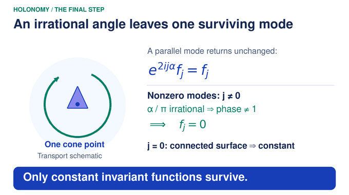
Zero gradient makes each coefficient parallel: locally constant, with constants matched by the chart transition phases. Now the angle hypothesis finally enters. Carry a coefficient around the cone corresponding to . The accumulated rotation, called holonomy, imposes:
For , irrationality of prevents the phase from equaling one. Every nonzero angular mode therefore disappears. The remaining coefficient is constant because the regular double is connected. Fourier completeness makes constant almost everywhere.
For an invariant indicator, a constant can only be zero or one. That closes the ergodicity of triangular billiards argument. It also explains why a rational right angle does not obstruct the theorem when the other two angle ratios are irrational. The analytic estimates themselves never needed an irrationality assumption.
10. Why Earlier Simulations Suggested Some Irrational Triangles Were Nonergodic
The 2022 study of symmetry in triangular billiards reported evidence that symmetric configurations might fail ergodicity, despite apparent correlation decay in typical triangles. The September manuscript also discusses earlier computations for irrational right triangles.
Finite trajectories can look localized for a long time. Such observations do not construct a positive-measure invariant set, and the new proof supplies no waiting-time estimate after which simulations must look uniform. This is where the verification discipline discussed in BootLoops’ scientific computing workflow matters: a numerical diagnostic and a theorem answer different questions.
A developer testing this system should track joint position and direction, document precision and corner handling, and avoid treating one initial condition as representative. Numerical angle approximations also cannot certify exact irrationality. Ergodicity does not prove that every orbit is typical, nor does it settle the separate existence question for periodic trajectories.
11. What the Proof Establishes for Quantum Billiards and What Remains Unproved
For quantum ergodicity triangular billiards now have a classical input to established spectral theorems. Corollary 7 applies to every Dirichlet or Neumann Laplacian eigenbasis on a qualifying triangle. A density-one subsequence means the proportion of retained indices among the first N tends to one.
| Conclusion | Qualification |
|---|---|
| Interior quantum ergodicity | Density-one equidistribution tested by observables supported away from the boundary |
| Boundary quantum ergodicity | Density-one convergence for boundary Cauchy data, with boundary-condition-dependent weights |
| Nodal domains | Counts tend to infinity along a density-one subsequence for real eigenbases |
| Not established here | Quantum unique ergodicity, quantitative rates, or a spectral-statistics law |
Density one is substantial, but it still allows an infinite exceptional subsequence. It does not say every highly excited state becomes uniform. The subsequences can depend on the triangle, boundary condition, and chosen eigenbasis. The paper obtains these conclusions by checking established spectral theorems’ hypotheses, rather than deriving a new spectral law from trajectory plots.
Boundary values require care: Dirichlet data use the normal derivative scaled by inverse frequency, whereas Neumann data use the boundary trace. Their limiting weights differ. These conclusions concern eigenfunction distribution, distinct from the energy-gap claims in our Laughlin spectral gap and two-dimensional area-law explainers.
The October 5 companion manuscript strengthens the classical claim to weak mixing. That still does not establish strong mixing. The Lean scope document describes classical ergodicity and flow construction, but its linked comparator theorem ends in sorry, an admitted placeholder. That file is not a completed certificate. We have not built a full Lean development or independently verified every analytic step. The distinction also matters in Lean proof verification elsewhere: a declared theorem and a checked proof are different evidence.
For irrational triangular billiards, the central contribution is the route from rough invariants through localized estimates and successive limits to holonomy rigidity. It offers no faster simulator or practical AI benchmark. Follow Binary Verse AI for research explanations that make the mathematics, assumptions, and verification evidence inspectable.
What are irrational triangular billiards?
Irrational triangular billiards describe a point particle moving in straight lines inside a Euclidean triangle and reflecting from its sides with equal angles of incidence and reflection. At least one interior angle must be an irrational multiple of π. Because the angles sum to π, at least two angle ratios are then irrational.
Did OpenAI’s proof establish ergodicity for every irrational triangle?
The September 25, 2026 manuscript presents a proof for every nondegenerate Euclidean triangle with at least one angle irrational relative to π. For normalized area times uniform direction, every measurable invariant set has probability zero or one, with no genericity or Diophantine condition. This describes the manuscript’s theorem, rather than independently reproduced verification of its entire proof.
Why was the ergodicity problem difficult to solve?
Earlier results covered generic families or tables satisfying strong rational-approximation conditions. An analytic approach also established constancy under a horizontal Sobolev regularity assumption that arbitrary bounded invariant indicators need not satisfy. The September argument works directly with bounded invariants and derives the coefficient regularity it needs.
How does OpenAI’s proof establish ergodicity?
The manuscript unfolds reflections onto the triangle’s flat double and decomposes invariant functions into angular Fourier modes. A localized energy estimate supplies individual square-integrable coefficient gradients. Cone-avoiding long trajectories and two successive limits force those gradients to vanish. Irrational rotational holonomy then eliminates nonzero modes, leaving only constant invariant functions.
Why did numerical experiments suggest irrational triangular billiards might not be ergodic?
Computations for some symmetric or irrational right triangles suggested nonergodicity or localization. Finite-time observations do not establish a positive-measure invariant set and can be consistent with very slow convergence. The manuscript gives a measure-theoretic argument, without a quantitative rate that would tell simulations when uniform statistics should emerge.
Does ergodicity prove that every triangular billiard has a periodic trajectory?
No. Ergodicity concerns invariant measurable sets and almost-everywhere time averages for a specified measure. A periodic trajectory returns exactly to its starting position and direction, which is a separate existence question. Vertex-hitting trajectories form a measure-zero exceptional set excluded from the theorem.
Does the proof also establish mixing and quantum ergodicity?
The September manuscript derives interior and boundary quantum ergodicity along density-one subsequences and nodal-domain growth for real eigenbases. It does not prove strong mixing or quantum unique ergodicity. A separate October 5, 2026 companion manuscript presents a proof of weak mixing, a stronger classical property than ergodicity that still differs from strong mixing.