
Knowing the lowest-energy state of a quantum system does not tell you how cheaply it can be disturbed. For the Laughlin state, that missing guarantee has challenged mathematical physics for more than four decades. OpenAI’s September 24, 2026 paper presents a Laughlin spectral gap proof for the full fermionic Haldane interaction on expanding spheres: sufficiently large systems have an excitation gap of at least , in the paper’s normalization.
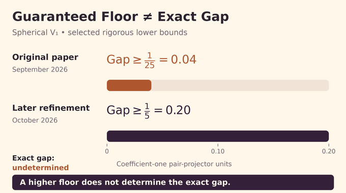
The advance is a lower bound covering every excited state, rather than another numerical estimate. A separate October refinement raises that floor to . To understand both results, start with the original argument: seven positive operator squares, exact finite certificates, and an error estimate that survives arbitrarily many particles.
Table of Contents
1. What Was the Laughlin Spectral Gap Conjecture?
A Hamiltonian is an operator whose eigenvalues are allowed energies. Its spectral gap is the separation between the ground energy and the next energy above the ground-state space. The Laughlin spectral gap conjecture asks whether this separation stays uniformly positive as the system grows.
At filling , particle number grows at roughly one third of the available magnetic orbitals. A positive gap for each finite system is insufficient: a sequence of smaller positive gaps could still converge to zero. The thermodynamic claim requires one lower bound that survives increasing size. Binary Verse AI’s Haldane gap explainer discusses the analogous uniformity question for a different model, a spin chain.
1.1. Laughlin Spectral Gap: Key Facts
| Feature | Original Paper’s Result |
|---|---|
| Interaction | Full fermionic pseudopotential, restricted to the lowest Landau level |
| Geometry | Round sphere, with a separate untruncated planar corollary |
| Laughlin Flux | for particles |
| Spherical Lower Bound | At least , for all sufficiently large particle numbers |
| Energy Convention | Coefficient one for each unordered-pair projector |
| Unspecified Quantity | An explicit particle-number or flux threshold |
2. Why the Laughlin Wavefunction Was Already an Exact Ground State
The spherical Laughlin polynomial is
Here are spinor coordinates for particle . The product runs over every unordered pair. Exchanging two fermions changes the sign, as antisymmetry requires. The cubic factor also forces a third-order zero when two particles coincide, suppressing the pair channel that the Hamiltonian penalizes.
This is a parent-Hamiltonian construction: choose an interaction for which the desired state has exactly zero energy. Every pair term annihilates the Laughlin state, so their sum does too. That fact was established long before this paper.
The logical trap is assuming that an exact ground-state formula automatically controls nearby energies. It does not. Other states could approach zero energy without ever becoming zero modes. Proving uniqueness identifies the bottom of the spectrum. Proving a uniform gap fences off everything immediately above it.
For example, three particles require six flux quanta. There are three cubed pair factors, and each particle appears in two of them, giving degree six in its coordinates. This degree bookkeeping explains why the special flux is tied to the polynomial rather than chosen merely for convenience.
3. The Spherical V1 Hamiltonian and Haldane Pseudopotentials
The original Fock-space paper studies
The operator acts on antisymmetric states in the lowest Landau level, the lowest magnetic kinetic-energy band. With flux quanta, its one-particle space has dimension and carries spin . The projector selects pair relative angular momentum one, equivalently pair spin .
Haldane pseudopotentials resolve an interaction into these pair channels. Keeping only the first fermionic channel defines the model. “Full” means retaining this complete interaction, including all its orbital couplings. It does not mean restoring every channel of the physical Coulomb interaction.
For the Haldane V1 pseudopotential, spectral gap comparisons require matching energy units. Each projector carries coefficient one. Multiplying the Hamiltonian by an energy scale multiplies its gap by that scale. At , the Laughlin polynomial has exactly the allowed degree in each particle. Keeping magnetic length fixed makes sphere radius grow proportionally to , producing a two-dimensional large-system limit.
Restricting to the lowest Landau level is part of the model definition. The theorem therefore studies the interaction within that band. It does not analyze transitions into higher Landau levels or prove that neglecting them is accurate for a particular experimental sample. Those physical questions require additional parameters and estimates.
4. Why Previous Approaches Could Not Prove a Uniform Laughlin Gap
Finite-size diagonalization can reveal a plausible gap, but even an encouraging sequence does not exclude a later collapse. Variational trial states answer another question: their excitation energies supply upper bounds. The missing theorem needs a lower bound for every orthogonal state.
Earlier rigorous results covered truncated pseudopotentials and special geometries, including thin-cylinder or thin-torus regimes. Those are substantive achievements with different hypotheses. A fixed-width cylinder does not become an expanding round sphere simply by adding particles.
There is another easily confused quantity: the entanglement gap concerns a spectrum extracted from a reduced state, rather than Hamiltonian excitation energies. Our 2D area law analysis explains why energy gaps and entanglement are connected, while remaining different mathematical objects.
The original paper’s contribution is control of the untruncated spherical interaction without a density-screening assumption. Its burden is global: no overlooked many-particle configuration may slip beneath the claimed floor.
The distinction is a worst-case guarantee. Testing a collection of candidate excitations can miss an unusual state with much lower energy. An operator lower bound covers that state too, whether or not anyone anticipated its structure or included it in a numerical search.
5. The Breakthrough: A Fock-Space Inequality Establishing a Positive Gap
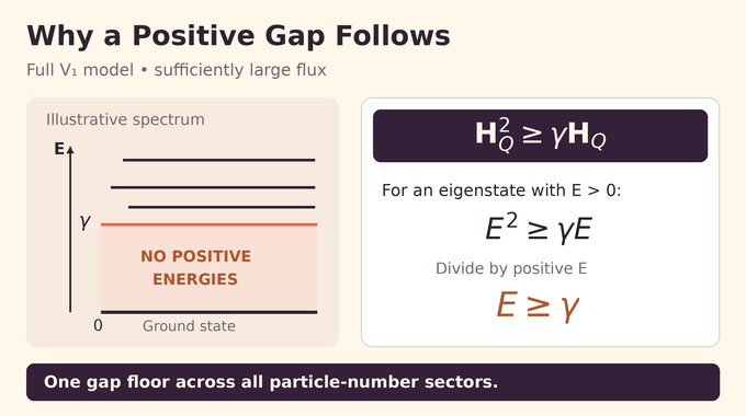
Instead of estimating individual excited states, the proof establishes an operator inequality on Fock space, the direct sum of all allowed particle-number sectors:
The inequality means that the difference has nonnegative expectation in every state. If an eigenstate has positive energy , it gives , hence . Zero-energy states remain allowed. The spectral interval between zero and is empty.
For every fixed , this holds once flux exceeds a threshold depending on , but not particle number. The original constant is , approximately , greater than .
One qualification matters. In a particle sector without a zero mode, this bounds the lowest energy away from zero. It does not necessarily separate that sector’s two lowest energies. At Laughlin filling, the unique zero mode makes it the usual excitation-gap statement.
This is research mathematics rather than a model leaderboard result. Our LLM math benchmark guide explains why test accuracy and a new theorem answer different evaluation questions.
As a simple check, a hypothetical energy of cannot satisfy the inequality with : its square is smaller than times its energy. The argument excludes every such low-energy eigenstate at once, without needing to construct or classify it.
6. Step One: Decomposing the Hamiltonian Square Into Few-Body Operators
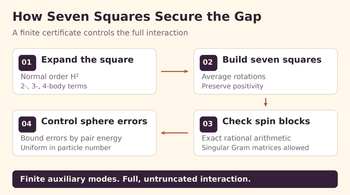
A pair-annihilation operator removes two particles in a specified interacting pair state. The Hamiltonian becomes a sum of its adjoint times itself. Each contribution is positive because its expectation is a squared norm.
Squaring that sum produces overlapping pair interactions. Normal ordering moves creation operators to the left using fermionic anticommutation. Two contractions leave a two-body term, one leaves a three-body term, and none leaves a four-body term. Exterior algebra, whose wedge products encode antisymmetry, organizes the signs and multiplicities.
The two-body contribution is the original Hamiltonian. The four-body contribution is positive. The three-body contribution contains the difficulty: its spin blocks can have negative coefficients, so positivity cannot be read off term by term.
The decomposition is exact on every particle sector. Positivity-preserving lifts carry few-body matrices into the full many-particle space. Rather than diagonalizing an enormous Hamiltonian, the proof asks which manageable operator inequalities will remain valid after this lifting. The algebra is doing the compression, without approximating away the interaction.
7. Step Two: Constructing Seven Positive Squares Using Rotational Symmetry
The authors introduce seven auxiliary operators, labeled . Each combines a pair annihilator with a term that removes a pair while moving another particle between orbitals. Those pieces have matching angular-momentum weight, allowing their cross terms to adjust the troublesome three-body contribution.
Summing produces a positive operator. Averaging its rotations over , the symmetry group describing spherical angular momentum, gives the positive comparison operator . Rotation averaging distributes the construction over the sphere without sacrificing positivity.
Only orbital modes zero through eight occur in the auxiliary squares. This finite support makes their coefficients tractable. It does not truncate the original Hamiltonian, whose pair interactions remain intact throughout the comparison.
The strategy has a price. The helpful three-body corrections consume some two-body energy, and four-body comparisons require a small allowance. A successful certificate must leave a positive balance after paying both costs. Seven squares are an explicit construction that works, not a theorem that seven is optimal.
8. Step Three: Reducing the Proof to Exact Spin-Block Inequalities
Rotational symmetry splits the three-body problem into angular-momentum blocks with explicit Gram eigenvalues. A Gram matrix records inner products between constructed vectors. In the four-body calculation, the same total spin can occur multiple times, so matrices between those copies must also be retained.
Some Gram matrices are singular. Inverting them would be invalid. The paper instead tests positivity after the coupling vectors are wedged into the physical four-fermion space. Null directions remain harmless rather than being silently discarded through an unjustified inverse.
8.1. What the Finite Certificate Checks
| Component | Exact Task |
|---|---|
| Seven Coefficient Rows | Integer row data determine the auxiliary operators and rational comparisons. |
| Three-Body Blocks | Strict inequalities cover indices two and four through fifteen. The wedge map kills indices zero, one and three. |
| Four-Body Blocks | Positive semidefiniteness is checked for twenty-three spin-deficit blocks, with singular Gram matrices allowed. |
A singular Gram matrix can simply mean that different coupling descriptions represent the same physical vector, or that a wedge vanishes. Positivity must be tested on those physical images, not demanded on an artificially independent list.
Appendix A supplies integer and rational arithmetic for these checks. Characteristic-polynomial coefficient signs certify the symmetric matrices’ positivity. Floating-point eigenvalues are not the final justification.
This separation between producing an argument and checking its certificate also matters in AI proof-verification workflows. OpenAI publishes a Lean solution module for the Fock-space theorem, alongside the mathematical exposition.
9. Step Four: Controlling Finite-Sphere Errors Uniformly
Exact positivity in a limiting matrix is not enough. The physical theorem concerns finite spheres, and the limiting Gram matrices have kernels. Small coefficient errors could become dangerous when lifted to a growing many-particle space.
The repair is an exact diagonal change of variables relating finite-sphere pair coefficients to their limiting values. On a fixed collection of modes, this transformation approaches the identity. Crucially, its error is bounded by local pair energy, so it vanishes on zero modes.
Adding spectator modes and averaging rotations then preserves control independent of particle number. An error proportional merely to the norm of an arbitrary state would not provide that protection.
This is why uniformity is the technical centerpiece. More particles mean more interacting pairs and more possible error contributions. Showing that a fixed small matrix converges is easy compared with proving that its lifted errors remain affordable in every sector. Pair-energy control supplies that missing accounting rule.
The remaining high-spin three-body terms form a summable tail, controlled by exponentially decaying coefficients. Combining the finite comparisons, their allowances, and that tail gives
Here is positive and tends to zero with increasing flux, uniformly across particle sectors. Choose any coefficient strictly below the limiting constant, then take flux sufficiently large. This is the bridge from finite certificates to an unlimited system size.
10. What the Proof Establishes for the Laughlin Ground State and Excitations
Zero energy forces every pair projector to vanish. Fermionic antisymmetry permits odd relative channels, so excluding channel one forces every pair bracket to divide the polynomial cubically. Their product exhausts the degree available at Laughlin flux, leaving only a constant multiple of the Laughlin state.
Combining that known uniqueness argument with the new inequality yields
Here projects onto the Laughlin ground-state line. The original Laughlin spectral gap lower bound is therefore a guarantee for all sufficiently large systems, not an exact gap value.
Corollary 6.3 also compares the neutral gap, at fixed particle number, with the particle-number charge gap at the same flux:
The charge gap is the second difference of ground energies when adding and removing one particle. It is not a transport measurement.
For the status as of October 14, Qiang Gao’s October 8 refinement raises the rigorous spherical floor to through sharper estimates and a larger semidefinite-programming certificate. It credits Claude Opus 5.5 under Gao’s direction. That subsequent improvement preserves the original architecture. It neither changes what the September paper proved nor determines the exact gap.
11. The Planar Corollary and the Exact Limits of the Proof
On the infinite plane, the original paper obtains the endpoint itself:
The bound holds uniformly in particle number and total angular momentum for the untruncated planar interaction. The proof takes the sphere-to-plane limit on each fixed homogeneous polynomial sector, then approaches the endpoint coefficient. It controls energy above the entire zero-mode space, which need not be a single line.
The published Lean scope documentation covers spherical and planar inequalities. Comparator files contain placeholder targets linked to separate solution modules. This article did not independently rebuild them. As our Fermat formalization explainer and percolation proof analysis emphasize, formalization and independent mathematical assessment are distinct checks.
The September theorem gives no explicit finite-sphere threshold, no full Coulomb gap, and no guarantee under arbitrary disorder. A separate companion addresses weak bounded projected scalar potentials. Nor does this paper benchmark quantum hardware or provide a quantum-computing speedup.
A gap theorem also does not supply an efficient procedure for preparing the ground state or simulating its excitations. It certifies an energy separation. Turning that separation into an algorithm, a device specification, or a measurable prediction is further work with its own assumptions.
For developers exploring automated mathematics, Appendix A offers a concrete reproduction target: implement the rational checks, preserve the printed normalization, and compare the resulting margins. Searching for better coefficients and certifying those coefficients are separate tasks. The October follow-up demonstrates how that separation can support further improvement.
Released within OpenAI’s October mathematics collection, the result illustrates why AI mathematical proofs need theorem-by-theorem reading. The useful lesson of the Laughlin spectral gap proof is its reusable certificate structure. Follow Binary Verse AI for research explainers that trace ambitious claims back to their equations, assumptions, and checkable evidence.
What is the Laughlin spectral gap conjecture?
It asks whether excitation energies above the Laughlin ground-state space stay bounded below by a positive constant as particle number grows. The September paper establishes this for the full spherical fermionic pseudopotential at filling , with coefficient one per pair projector.
Why was the Laughlin spectral gap difficult to prove?
The Laughlin wavefunction was already known to be an exact zero-energy ground state. The difficult step was bounding the energy of every orthogonal state below by one fixed positive constant, independently of particle number. Finite-size numerics and variational upper bounds cannot establish that universal lower bound.
How does OpenAI’s proof establish the Laughlin spectral gap?
The proof decomposes the Hamiltonian square into few-body terms and compares them with rotational averages of seven positive operator squares. Exact spin-block certificates and a particle-number-independent error estimate establish . A positive eigenvalue must then satisfy .
Is the Laughlin spectral gap exactly ?
No. The September paper proves a lower bound of for sufficiently large spherical systems in its coefficient-one pair-projector normalization. It does not determine the exact excitation gap. Qiang Gao’s October 8, 2026 preprint subsequently raises the rigorous spherical lower bound to .
Does the proof work for the full Haldane interaction?
Yes. It treats the complete spherical pair-projector Hamiltonian rather than a truncated orbital-chain approximation. Its auxiliary positivity construction uses finitely many orbital modes, but the interaction being bounded remains untruncated. Full does not mean the full Coulomb interaction.
Does the Laughlin spectral gap proof also apply to the infinite plane?
Yes. The original paper’s planar corollary bounds the positive spectrum of the untruncated planar Hamiltonian below by , uniformly in particle number and total angular momentum. The bound is above the entire zero-mode space. It does not establish a gap for the complete physical Coulomb interaction.
Has the Laughlin spectral gap proof been formalized in Lean?
Yes, according to the published Lean documentation, which describes spherical Fock-space and planar gap inequalities. The repository links comparator targets to separate solution modules. Their publication is distinct from an independent audit or successful external rebuild, neither of which was performed for this article. The documented scope does not formalize stability under projected one-body potentials.