

Randomness was supposed to set the floor. For every bipartite pattern, the Sidorenko conjecture predicts that a graph with a given edge density contains at least the pattern density supplied by a uniformly random model. OpenAI’s manuscript claims that a carefully arranged graph can slip beneath that floor.
The proposed Sidorenko conjecture counterexample has 35 vertices and 66 edges. The paper specifies this pattern exactly and proves the existence of a finite simple host graph in which its normalized homomorphism count violates the predicted inequality. It also derives a counterexample to the related forcing conjecture.
That answers the central search question early: OpenAI reports a disproof, with supporting Lean material for the main finite-host statement. Understanding the result still requires separating the pattern from its host, the manuscript from independent verification, and the main theorem from its consequences.
Table of Contents
1. What the Sidorenko Conjecture Counterexample Actually Claims
The September 23, 2026 manuscript, A counterexample to Sidorenko’s conjecture, states its main result as Theorem 1.1. For the specified bipartite graph H, some finite simple undirected graph G with at least one edge satisfies
t(H,G) < p(G)66.
The attached manuscript supplies the construction and argument: OpenAI, 2026.
Sidorenko Conjecture: Key Facts About the 35-Vertex Counterexample
| Key Fact | What the Paper States | Why It Matters |
|---|---|---|
| Pattern size | 35 vertices, 66 edges | These numbers describe H, not the host |
| Pattern construction | Incidence graph of 22 triples on 13 points | Readers can reconstruct its adjacency |
| Host | Existence of a finite simple graph G | The conclusion reaches ordinary graphs |
| Counting convention | All edge-preserving vertex maps | Repeated vertex images are included |
| Further consequence | Failure of forcing at one positive density | Matching two densities can miss structure |
A drawing of 35 vertices therefore isn’t the complete counterexample certificate. The violation concerns how that pattern occurs inside another graph. The proof constructs weighted models first, then transfers a strict deficit to a finite host through sampling.
2. The Original Inequality and Its Random-Graph Benchmark
The Sidorenko conjecture formula is
t(H,G) = hom(H,G) / |V(G)||V(H)| ≥ p(G)|E(H)|, p(G) = 2|E(G)| / |V(G)|2.
A homomorphism sends vertices of H into G while preserving edges. Different source vertices may share an image. Extra host edges are allowed, so this doesn’t count induced copies.
Sidorenko Conjecture: Key Mathematical Quantities and Their Meanings
| Quantity | Plain-English Meaning | Convention to Remember |
|---|---|---|
| hom(H,G) | Number of edge-preserving maps | Maps needn’t be injective |
| t(H,G) | Probability a random vertex map preserves every edge | Divide by all vertex maps |
| p(G) | Probability two independent vertex draws are adjacent | Uses n2, including repeated draws |
| p|E(H)| | Pattern density in a constant kernel of mean p | The conjectured lower benchmark |
| Injective copies | Maps using distinct host vertices | Require a separate finite-size normalization |
If the density is p, an independent-edge benchmark assigns a factor p to each required edge. For this pattern, that gives p66. The exact comparison uses a constant weighted kernel. Finite random graphs approach that benchmark as their order grows.
The intuition works for simple patterns. For a two-edge path, its density is the average squared normalized degree. Nonnegative variance makes this at least the square of the average degree. The proposed construction exploits correlations that this elementary argument cannot see.
For a finite host, the usual edge density divides by the number of distinct unordered vertex pairs. That differs slightly from the paper’s convention. The two agree asymptotically, but switching denominators mid-calculation can change a claimed finite violation.
3. Why Earlier Positive Results Still Matter
The Sidorenko inequality holds for important families, including trees, even cycles, and complete bipartite graphs. Broader methods cover weakly norming graphs, graphs with a vertex adjacent to the entire opposite part, and constructions meeting specific gluing, subdivision, or degree-count conditions.
Those results remain valid under their hypotheses. A counterexample to the universal claim identifies where those hypotheses stop being enough.
OpenAI’s incidence graph has point-side degrees 4, 5, and 6, while every triple-side vertex has degree 3. Neither side contains a vertex joined to the whole opposite side. Its irregular point side also excludes the necessary regularity condition for a connected weakly norming graph.
The manuscript checks that cited degree-count criteria fail in both orientations. Its minimum degree is 3, so it also lacks the degree-2 vertices introduced by the specified even-path substitution constructions.
A further subtlety concerns blow-ups. Some positive theorems establish the inequality after sufficiently enlarging one side of a pattern. That doesn’t establish it for the original pattern. Changing the graph changes the question.
Local versions also survive: the manuscript cites conditions under which kernels sufficiently close to a constant satisfy the inequality. A global counterexample can coexist with a protected neighborhood around the random benchmark. Its normalized kernel must escape those local hypotheses.
4. Inside the 35-Vertex, 66-Edge Graph
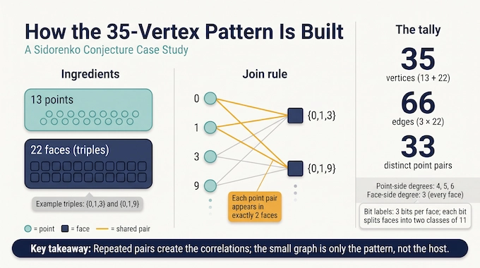
Start with 13 points and 22 three-element subsets, called faces. Create one vertex for each point and one for each face. Join a point to a face exactly when that point belongs to the triple.
The arithmetic is straightforward: 13+22=35 vertices and 3×22=66 edges. The two vertex sets are separate, even when their numerical labels coincide.
The underlying triples contain 33 distinct point pairs, each appearing in exactly two faces. For example, the triples {0,1,3} and {0,1,9} share the pair {0,1}. Connecting faces that share a pair produces a connected face-neighbor graph.
Table 1 also assigns three bits to each face. Every bit position splits the faces into two classes of 11, each covering all 13 points with a prescribed exposure order. Faces sharing a pair differ in at least one bit position.
These labels help control the later estimates. The repeated pairs create the correlations, while connectivity lets local constraints propagate through the whole construction. The small graph supplies a tightly organized framework for a much larger algebraic model.
5. How Repeated Pairs Preserve Hidden Correlations
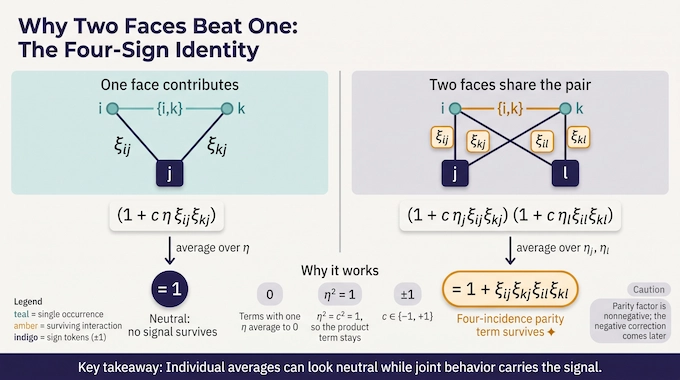
The central identity fits on one line. Let a point pair {i,k} occur in faces j and l. Attach incidence signs ξ, each equal to +1 or -1, and average over an independent uniform sign η:
Eη[(1 + cηξijξkj)(1 + cηξilξkl)] = 1 + ξijξkjξilξkl,
where c ∈ {−1, +1}.
Terms containing one factor of η vanish because its average is zero. The product survives because η2=c2=1. If only one face contributes, the average is simply 1.
Consequently, activating both face occurrences preserves a four-incidence parity interaction that a single occurrence cannot produce. Individual averages can look neutral while their joint behavior carries a signal.
This identity alone doesn’t violate the conjecture. Its parity factor is nonnegative. The negative correction emerges later, when carefully chosen activation distributions combine these surviving interactions. The mathematical task is to make that correction survive every other contribution to the full density.
6. Why Symmetric Matrices Enter the Proof
The OpenAI Sidorenko conjecture construction realizes that sign model using symmetric matrices over Fq, where q is an odd prime.
Fix a sufficiently large even dimension D=2r. For a matrix difference, the construction selects rank r and a discriminant sign. This sign records whether the determinant of the induced nondegenerate quotient form is a square or nonsquare in the field.
Selecting a rank-and-sign layer, then dividing its indicator by its probability, produces a nonnegative factor with mean one. That normalization keeps the edge average controlled while allowing higher-order interactions.
Half rank supplies the geometric constraint. When two point matrices have a nonsingular difference, the rank-r images through a common center are complementary, linking their discriminant signs.
The rank-layer lemma states that the averaged matrix products approach the required parity model. A joint estimate supplies asymptotically independent signs on all 33 point pairs. Crucially, the dimension and other construction parameters are fixed before q grows. Letting every parameter drift together would require a different justification.
7. Activation Laws Make One Negative Contribution Dominate
A sampled vertex receives a type indicating which point or face it is intended to represent. Independent matrix coordinates carry copies of the rank-layer model, while activation laws determine which coordinates participate at each type pair.
Two activation branches carry opposite sign biases. Their nonconstant first sign moments cancel, but an overlap moment survives. This creates room for a signed higher-order correction without altering the controlled mean.
At the intended type assignment, the support constraints permit exactly one labeling with every pair label nonempty. Choosing one incidence corner to carry a negative sign makes its coefficient
−(θ/2)66, 0 < θ < 1.
Other assignments remain a problem, including maps that repeat types. The manuscript uses scores derived from color refinement, which repeatedly distinguishes vertices by their neighbors’ colors. For this graph, refinement eventually separates all vertices within each part.
Those scores make the intended assignment dominate competing assignments in the weighted sum. This step matters because an unfavorable coefficient inside an expansion isn’t yet an unfavorable total density. The proof must win after every allowed map is counted.
Throughout this process, the actual kernel weights remain nonnegative. The minus sign belongs to a correction in the expanded expectation. Confusing those two levels would turn the construction into a different problem, since negative edge probabilities cannot define the host used in the theorem.
8. The Singular Configurations Cannot Be Swept Aside
The hardest obstacle is that some point-matrix differences are singular. Their probability is O(q−1), which sounds harmless until the normalized rank indicators enter the calculation.
Those indicators can grow as powers of q. A rare event multiplied by a large weight may still dominate an expectation. Probability alone doesn’t settle its contribution.
Sections 5–7 replace the matrix problem with Lagrangian geometry. For a symmetric matrix X, the subspace
LX = {(v, Xv) : v ∈ FqD}
is Lagrangian in the relevant symplectic space. The intersection LX ∩ LY corresponds to the kernel of X-Y, turning rank defects into intersection dimensions that can be counted.
The argument balances the cost of an intersection profile against the gain from conditioning on face centers. It then treats remaining cases through propagation constraints and additional span counts.
This is where the intuitive mechanism becomes a demanding proof. The four-sign identity explains the intended effect. The singular bounds establish that exceptional configurations don’t erase it. Any serious reading of the Sidorenko conjecture proof must follow both branches.
9. From Weighted Kernels to an Ordinary Finite Graph
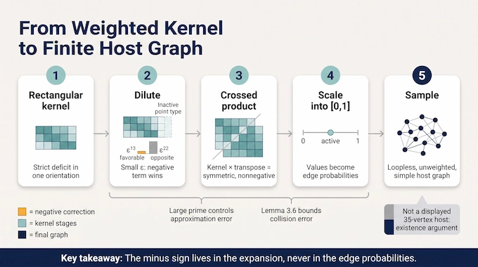
The first strict deficit appears in one orientation of a rectangular kernel. Reversing its two spaces can introduce an uncontrolled correction, so the proof adds an inactive point type.
After this dilution, the favorable correction scales as ε13, while the opposite correction scales as ε22. For sufficiently small positive ε, the negative term dominates. A sufficiently large prime then controls the remaining approximation error.
The construction next combines the kernel with its transpose in a crossed product. This yields a symmetric nonnegative kernel. Scaling its values into [0,1] preserves the normalized density comparison, allowing those values to serve as edge probabilities.
Sampling labels and edges produces ordinary finite simple graphs. The strict gap survives the error from source-vertex collisions. Lemma 3.6 bounds that collision contribution explicitly, retaining all homomorphisms in the final count.
The conclusion therefore concerns a loopless, unweighted host graph. Still, the manuscript’s explicit small object is the pattern. Its existence argument for the host shouldn’t be advertised as a displayed 35-vertex host with a directly tabulated deficit.
10. Tensor Powers Amplify the Violation
Suppose the resulting host satisfies
ρ = t(H,G) / p(G)66 < 1.
In a categorical tensor power G×k, vertices are tuples and adjacency must hold in every coordinate. Homomorphism and edge densities multiply coordinatewise, giving
t(H,G×k) / p(G×k)66 = ρk → 0.
Thus the same pattern can fall below any prescribed positive multiple of the benchmark. One strict violation leads to arbitrarily large multiplicative failures.
The qualification is density: p(G×k) = p(G)k, so the host density changes and tends to zero.
A separate balanced blow-up argument establishes a fixed deficit in injective labeled copies at one positive limiting density. Replace each host vertex by an equally sized independent set and each host edge by a complete bipartite connection between the corresponding sets. Homomorphism density stays fixed, while the relative collision error vanishes as the sets grow.
These are distinct consequences. Arbitrarily strong relative failure with varying density doesn’t automatically establish arbitrarily strong failure at every fixed density.
11. The Forcing Conjecture Consequence
The forcing conjecture asks whether matching a random model’s edge density and one suitable bipartite pattern density forces a graph sequence to be quasirandom. Quasirandomness means matching the limiting densities of every fixed finite pattern.
The manuscript derives a forcing conjecture counterexample from the same connected cyclic graph. At one fixed p∈(0,1), it constructs a nonconstant graphon W satisfying
t(K2,W) = p, t(H,W) = p66.
The mechanism is interpolation. One kernel lies below the pattern benchmark. Another kernel with the same mean lies above it. Moving continuously between them reaches equality, while an independent-coordinate argument keeps the interpolated kernel nonconstant.
Its four-cycle density is strictly greater than p4. Sampling then gives finite graphs whose edge and H-densities converge to the random benchmarks, yet whose four-cycle density exposes persistent structure.
Equality in these two measurements can therefore conceal nonrandom organization. The result supplies one density where this pattern fails to force quasirandomness. It doesn’t assert failure at every density or invalidate the classical edge-and-four-cycle characterization.
12. Verification, Minimality, and What to Read Next
As of October 11, 2026, OpenAI’s repository describes a Lean formalization for the specified finite-host counterexample. Its scope page explicitly excludes the separate forcing-conjecture consequence from that statement. Saying the paper has no formal support would miss this distinction.
A published formalization and an independently reproduced verification run provide different evidence. This article reports the manuscript and documented scope. It doesn’t certify a fresh Lean run or independent referee acceptance. OpenAI also describes the collection as model-produced work at different verification stages.
The paper doesn’t establish that 35 vertices is globally minimal. It establishes a particular construction. Excluding every smaller bipartite pattern would require another argument.
For readers searching “Sidorenko conjecture disproved,” the precise takeaway is a claimed universal counterexample with formalization material covering the main statement. Its force comes from controlled correlations, careful exceptional-case bounds, and a transfer to ordinary finite graphs.
Read the original paper, starting with Theorem 1.1 and the proof-dependency diagram. Follow Binary Verse AI for further analysis of the Sidorenko conjecture, with verification scope kept visible alongside the mathematics.