
AI runs on an extraordinary amount of matrix multiplication. Training models, processing attention and transforming hidden representations all depend on combining grids of numbers efficiently. A better mathematical bound for that operation deserves attention, even when it doesn’t arrive with a CUDA kernel attached.
The OpenAI Matrix Multiplication paper, dated October 2, 2026, establishes an upper bound of 9/4, or 2.25, for the exponent of square matrix multiplication over complex numbers. It appeared in the research collection OpenAI released on October 6, produced by an internal frontier model.
The precise claim is that, for every positive ε, two n×n complex matrices can be multiplied using Oε(n²·²⁵⁺ε) arithmetic operations. The paper doesn’t establish a competitive matrix size or demonstrate faster AI training. Its significance lies in the proof: a new separation construction connects polynomial multiplication to a substantially lower ceiling on matrix multiplication complexity.
Table of Contents
1. What OpenAI Matrix Multiplication Actually Establishes
The central number is ω, pronounced omega. It describes the best asymptotic arithmetic exponent achievable for matrix multiplication in the specified number system.
OpenAI Matrix Multiplication: Key Findings and Proof Scope
| Key Fact | What It Means |
|---|---|
| Paper | An Upper Bound of 9/4 for the Matrix Multiplication Exponent |
| Main Claim | ω(ℂ) ≤ 9/4, or 2.25 |
| Operation Bound | Oε(n2.25+ε) for every ε > 0 |
| Matrices Covered | Two n×n matrices over complex numbers |
| Computational Model | Scalar arithmetic operations |
| Practical Evidence | No competitive finite-size implementation established |
| Formalization | The repository includes a Lean theorem for the complex 9/4 bound |
An upper bound establishes what’s achievable in principle. It doesn’t prove that 2.25 is optimal. A smaller exponent might still be possible.
The ε matters too. The statement permits an arbitrarily small positive addition to 2.25, with an algorithm and constants that can depend on that choice. Dropping ε makes a convenient headline, but changes the literal guarantee.
That distinction prevents a common mistake: reading an asymptotic existence theorem as a fixed performance specification.
2. Why Matrix Multiplication Time Complexity Matters
Each entry of a matrix product is a row-column dot product. For example, combining the row [2, 3] with the column [4, 5] produces 2×4 + 3×5 = 23.
For n×n matrices, the conventional method computes n² output entries, each involving roughly n multiplications and additions. That produces cubic arithmetic growth, O(n³).
Changing the exponent changes how rapidly the work increases as matrices grow.
OpenAI Matrix Multiplication: Exponent and Scaling Comparison
| Method or Bound | Exponent | Illustrative Work Increase When n Doubles |
|---|---|---|
| Conventional Multiplication | 3 | 8× |
| Strassen Algorithm | About 2.807 | 7× |
| AlphaEvolve-Assisted Bound | Below 2.371177 | About 5.17× at the quoted exponent |
| OpenAI Complex Bound | At Most 2.25 | About 4.76× at the headline exponent |
These are exponent-only illustrations. They omit constants, ε slack and lower-order work. They aren’t measured speedups.
GPUs introduce another distinction. Parallel hardware can perform many operations simultaneously, improving elapsed time without necessarily changing the arithmetic exponent. Arithmetic complexity also treats scalar operations as individual steps. It doesn’t automatically account for the bit-level cost of representing numbers accurately.
The theorem changes a mathematical scaling limit. Hardware performance requires additional evidence.
For a fair comparison, ask what is being held constant. Multiplying larger matrices on the same machine differs from adding more processors, reducing numerical precision or approximating the answer. All can change performance, but they don’t establish the same theorem. This paper concerns exact multiplication in an arithmetic model, with matrix size tending to infinity.
3. From Strassen To AlphaEvolve: Why 2.25 Is Significant
The Strassen algorithm showed in 1969 that ordinary multiplication wasn’t the final answer. Two 2×2 matrices can be multiplied using seven scalar multiplications rather than eight, with additional additions and subtractions.
Apply that identity recursively to matrix blocks and the exponent becomes log₂7, approximately 2.807. The insight was structural: reorganizing the computation could beat the obvious row-by-column procedure.
Later work developed tensor methods, including the laser method and increasingly sophisticated analyses of tensor powers. The August 2026 AlphaEvolve-assisted paper reported ω < 2.371177, improving the preceding 2.371339 bound through optimization and combination-loss analysis.
The OpenAI Matrix Multiplication result moves the complex upper bound substantially further, to 2.25, through a different argument involving tensor characters and polynomial multiplication.
The AlphaEvolve-Strassen comparison also needs care. Discovering an improved formula for a particular small matrix size and improving the asymptotic exponent are related achievements, but they answer different questions. One concerns a finite construction. The other concerns scaling across arbitrarily large sizes.
4. Which Number Systems And Matrix Shapes Are Covered?
The headline theorem is stated over ℂ, the complex numbers. It should not be silently rewritten as a theorem with the same exponent over every field.
The collection includes a separate every-field bound, ω(F) < 2.371054886006746. That result includes finite fields and positive characteristic. Its broader scope comes with a different numerical bound.
Companion results also address rectangular multiplication. The formalization documentation lists a dual exponent greater than 0.465 and a bound below 2.092 for multiplying n×n⁰·⁷⁰⁹ by n⁰·⁷⁰⁹×n complex matrices.
The dual exponent asks how large the inner dimension can grow while multiplication remains near quadratic in the outer dimension. That makes it relevant to understanding rectangular computations.
However, those companion results are not all proved in the October 2 manuscript. A careful OpenAI Matrix Multiplication explainer keeps the papers’ contributions separate rather than treating the repository as one enormous theorem.
5. The Proof’s Language: Tensor Rank And Characters
The proof encodes matrix multiplication as a trilinear expression, with one variable group for each input and another paired with the output. These three groups are called tensor legs.
Tensor rank measures the smallest number of simple trilinear products needed to express that tensor. In algorithmic terms, a rank decomposition provides a bilinear recipe: form linear combinations of input entries, multiply them, then combine the results.
Tensor characters provide a different tool. They assign numerical values to tensors while respecting three operations: combining independent problems, taking tensor products and reducing one tensor to another through linear substitutions.
Think of them as consistent measuring instruments. Each respects the same rules, although different instruments can return different values.
The proof needs more than convenient measurements. Its detecting-character lemma ensures that sufficiently large rank-based complexity would be visible to some character. The appendix establishes that existence result using separation, compactness and a fixed-point theorem.
This is the bridge from bounding all characters to bounding multiplication complexity itself.
6. The Key Construction: Separating A Shared Tensor Leg
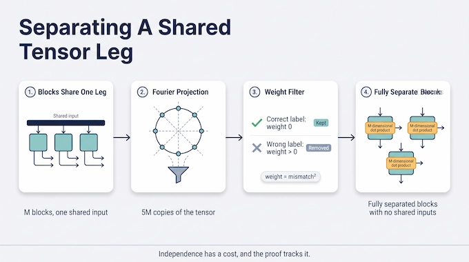
Useful tensor pieces often overlap. Imagine several blocks with separate second and third variable groups, but a shared first group. They look partly independent, yet cannot be treated as a full direct sum, which requires separation on all three legs.
The paper’s finite separation construction addresses precisely this obstruction.
It starts with M blocks and uses 5M copies of the source tensor. Linear substitutions involving roots of unity perform a finite Fourier projection. The shared first-leg variables receive tentative block labels, while the projection removes terms that fail an index-matching condition.
Next comes a degeneration, an algebraic filtering operation. Variables receive powers of a formal parameter, and the construction retains terms with minimum total weight.
The weights make a surviving term’s total weight equal the square of its label mismatch. Correct labels have weight zero. Incorrect labels have positive weight and disappear from the retained tensor.
The result has fully separated blocks, each carrying an auxiliary M-dimensional dot product. That extra factor matters: it supplies the gain used later. The construction does not create M² independent blocks, and confusing those multiplicities would break the argument.
For intuition, picture two blocks that both use an input called x. Merely renaming x separately inside each block would change the problem without justifying the change. The Fourier projection and weighting construction provide that justification algebraically, while accounting for the copies and auxiliary factors needed to accomplish it. Independence has a cost, and the proof tracks it.
7. How Polynomial Multiplication Forces The 9/4 Bound
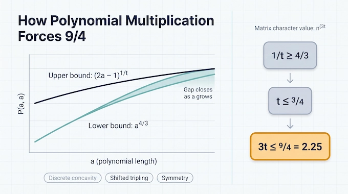
The separation construction becomes an entropy inequality after applying it to tensor powers. Counting words with prescribed block frequencies gives an exponential growth rate governed by entropy. Taking roots then turns that counting into a bound on character values.
The next target is ordinary polynomial multiplication. Two coefficient vectors of lengths a and b produce a coefficient vector of length a+b−1. Evaluation and interpolation give its tensor rank exactly a+b−1.
The paper combines character values across all six permutations of the tensor legs into a symmetric profile, P(a,b). Its normalization uses a positive parameter t derived from the character’s three dot-product exponents.
7.1. Two Constraints On The Profile
A determinant filtration compares neighboring polynomial lengths. It separates quotient and kernel pieces in bases compatible with every first-input multiplication map. That compatibility matters: the construction must work for the whole tensor, not merely one chosen input.
The resulting inequality makes P discretely concave. Increasing an input length produces increments that do not increase.
A separate three-sector construction divides the second-input and output coordinates into matched regions. Applying the separation inequality and averaging over leg permutations gives shifted tripling:
[ P(a,3h+a-1)\geq 3P(a,h). ]
Together with symmetry and P(1,b)=b, these constraints force substantial diagonal growth.
7.2. Where 2.25 Comes From
The discrete-growth lemma establishes:
[ P(a,a)\geq a^{4/3}. ]
Interpolation and the rank bound also give:
[ P(a,a)\leq(2a-1)^{1/t}. ]
As a grows, both inequalities can hold only if 1/t ≥ 4/3, meaning t ≤ 3/4. Matrix multiplication’s character value is n³ᵗ, so its exponent is bounded by 3t ≤ 9/4.
The detecting-character lemma then converts this universal character bound into the rank-based exponent bound. Polynomial multiplication supplies the constraints that make a larger exponent impossible within the argument.
8. From An Exponent Bound To An Algorithm
The last step turns the rank result into an arithmetic algorithm.
For a chosen positive ε, the proof establishes the existence of a fixed block size and an exact rank decomposition with sufficiently few products. Apply that bilinear identity recursively to larger matrix blocks, accounting for additions and scalar coefficients, and the required operation bound follows. Padding handles dimensions that aren’t exact powers of the block size.
This explains why calling the entire paper “nonconstructive” is too blunt. Its separation and polynomial constructions are explicit. However, the endpoint relies on existence of a suitable decomposition without displaying a competitive one.
The OpenAI Matrix Multiplication proof therefore establishes algorithmic possibility without supplying an implementation engineers can drop into a training stack.
“An algorithm exists” carries mathematical content. “Here is its code, memory use and benchmark” carries engineering content. The paper delivers the first kind of result.
9. Checking The Paper, GitHub And Lean Formalization
The October 2 manuscript provides the written argument. The OpenAI Matrix Multiplication GitHub materials also include formalization scope notes and the Lean theorem entry point.
The entry point states the complex 9/4 bound using the repository’s arithmetic-exponent definition. The scope notes distinguish that result from the every-field and rectangular claims.
Formal verification checks a precisely stated theorem against encoded definitions and proof rules. Expert review asks complementary questions: does the statement capture the manuscript’s intended claim, are dependencies appropriate, and how does the result relate to earlier work?
A published theorem file, a successfully checked build and a reviewed mathematical contribution are different pieces of evidence. A responsible reader examines the statement and its supporting definitions rather than treating a Lean label as a substitute for understanding.
That scrutiny is especially useful when the claimed improvement is this large.
10. Why The Bound Does Not Immediately Accelerate GPUs
For builders, the question is straightforward: will this make their workload faster?
The paper doesn’t answer that experimentally. Its arithmetic bound leaves practical crossover sizes unspecified. Constants and additional work can dominate at the dimensions people actually use.
Memory movement matters too. A method that reduces scalar products may require extra combinations, temporary storage or communication. Those costs affect performance on finite hardware.
Numerical behavior is another missing bridge. Exact identities over complex numbers don’t automatically establish floating-point stability at the precision used for training or inference. Real model workloads also involve rectangular shapes, batching and operations beyond matrix multiplication.
So, is Strassen’s algorithm used in practice? It can be, where dimensions and implementation tradeoffs suit it. That doesn’t establish that a much lower asymptotic exponent will outperform optimized conventional multiplication.
A “galactic algorithm” is one whose asymptotic advantage appears only at impractically large sizes. The phrase describes a legitimate concern here, but the manuscript doesn’t determine a crossover threshold. Assigning it one would be guesswork.
11. What Could Change For Algorithms And AI?
The immediate significance is theoretical. Algorithms whose running times depend on matrix multiplication’s exponent may inherit improved bounds when their reductions and computational assumptions match the new result. Each application still needs its own analysis.
The longer-term engineering opportunity is more demanding. Researchers would need useful decompositions, efficient implementations, precision analysis and performance measurements across relevant shapes and hardware. An end-to-end AI benefit would also depend on how much of the workload the improvement actually accelerates.
That is why dollar savings and energy reductions cannot be read off the exponent. Nor does the result prove ω=2. The usual quadratic lower bound reflects the scale of dense input and output, while the remaining gap is still unresolved.
There is an intriguing feedback possibility: AI-assisted mathematics could inform algorithms that improve future AI computation. But this paper doesn’t demonstrate a deployed self-improvement loop. It establishes a mathematical result that might become one ingredient in such a process.
12. What To Watch Next
The OpenAI Matrix Multiplication story now has three useful checkpoints: independent understanding of the proof, concrete decompositions that expose its algorithmic potential, and benchmarks showing whether any construction helps finite workloads.
For researchers, the separation method deserves close attention. For developers, the practical signal will be reproducible code with measured speed, memory use and numerical behavior. Until those arrive, the exponent is a reason to investigate, not a reason to rewrite production software.
Follow Binary Verse AI at binaryverseai.com for clear explanations of the proof reviews, algorithm developments and benchmarks that follow. The next important number may be 2.25’s theoretical successor. It may also be a measured runtime. Both deserve careful reading.
1. What did OpenAI prove about matrix multiplication?
OpenAI’s paper establishes an upper bound of 9/4, or 2.25, for the matrix multiplication exponent over complex numbers. More precisely, for every positive ε, two n×n complex matrices can be multiplied using \(O_\varepsilon(n^{2.25+\varepsilon})\) arithmetic operations. This describes asymptotic scaling; it does not establish a practical GPU speedup.
2. What is the Big O time complexity of matrix multiplication?
The standard algorithm uses O(n³) arithmetic operations for two n×n matrices. Strassen’s algorithm reduces this to approximately O(n²·⁸⁰⁷). OpenAI’s paper establishes the existence of algorithms approaching exponent 2.25 over complex numbers. Actual execution time also depends on constants, matrix dimensions, numerical precision and hardware.
3. Is OpenAI’s matrix multiplication proof verified in Lean?
OpenAI’s repository includes a Lean theorem stating that the complex matrix multiplication exponent is at most 9/4. Its documentation identifies this as an arithmetic-complexity result. Checking the formalization’s build, assumptions and correspondence with the manuscript remains distinct from peer review and practical performance testing.
4. Has OpenAI released a usable O(n²·²⁵) matrix multiplication algorithm?
The paper proves that algorithms exist with operation counts approaching exponent 2.25 and explains how a suitable bilinear decomposition yields recursive multiplication. However, it does not supply a competitive finite-size GPU implementation or establish where such an implementation would outperform existing methods.
5. Will this result make AI training and inference cheaper?
It could inform future algorithm research, but the paper establishes no immediate reduction in AI costs. Practical benefits require an efficient implementation, manageable overhead, appropriate memory behavior and numerical reliability. GPU benchmarks and complete workload measurements would be needed before estimating training, inference or energy savings.