
Introduction
If you’ve ever stared at a loss curve and thought, “Cool, it’s going down, but what did the model actually learn?”, you’re not alone. We’ve trained ourselves to treat lower loss like truth. But a model can get better at predicting text while learning almost nothing reusable, and it can also struggle early while quietly assembling a library of useful subroutines. Those two worlds look annoyingly similar if your only instrument is loss.
That’s why I’m excited about Epiplexity, a new way to talk about information that finally matches the reality of modern training. It starts from a blunt observation: information isn’t just “how random is the data.” It’s “how much structure a bounded learner can extract into its weights.” The paper introducing it frames the mismatch as three “paradoxes” where classical Information Theory in Machine Learning shrugs, while practice keeps shipping products anyway.
Table of Contents
1. The Paradox Of AI Learning: Why Noise Looks Like Information

Here’s the trap. Random noise has high Shannon Entropy. A perfect model can’t compress it. Yet random noise also teaches a model nothing beyond “don’t bother, it’s random.” Meanwhile, a dataset full of deep structure can have less raw randomness, but it can force a model to build complicated internal machinery. Classic metrics call both “information,” then wonder why training behaves weirdly.
The paper illustrates this with examples you’ve seen in the wild: configuration files stuffed with hashes and API keys, images with pixels shuffled, and other “hard to predict” junk that has tons of randomness but almost no learnable structure.
Epiplexity Data Types: Learnable Structure vs Noise
Fits the content area. Wraps text, no layout jitter.
| Data Type | Shannon Entropy Intuition | What A Training Run Feels Like | What The Model Keeps | What You Should Do |
|---|---|---|---|---|
| Pure random bits | Max randomness | Loss stalls near chance | Almost nothing reusable | Don’t waste compute |
| Pseudorandom outputs without the key | Looks random to bounded compute | Loss behaves like noise | Still nothing reusable | Treat as noise in curation |
| Natural text with long-range patterns | Mixed randomness and structure | Loss improves steadily | Reusable circuits, abstractions | Prioritize for training |
| Procedural worlds with emergent rules | Structure hides behind compute | Slow improvement, then insight | Compact “programs” of behavior | Great for capability growth |
| Hashes, IDs, file paths | Predictively painful | Loss stays stubborn | Mostly memorization | Downweight for LLM Optimization |
The punchline is simple. You’re not paying for randomness. You’re paying for the structural bits the model can internalize, then reuse.
2. What Is Epiplexity? Defining Structural Information

Classical information theory asks, “How many bits do I need to describe a sample if I already know the distribution?” That’s entropy, and it’s beautiful. But training doesn’t hand your model the distribution. Training hands it a finite dataset and a compute budget, then says: learn what you can.
Epiplexity is built around Minimum Description Length (MDL), which splits description length into model bits and data-given-model bits. The twist is the bounded part: the best model is the one that compresses the data well subject to a runtime limit.
Formally, the paper defines an optimal time-bounded probabilistic program (P^*) that minimizes “program length plus expected negative log-likelihood.” Then:
- the Epiplexity of the data is the length of that optimal program, the structural bits,
- the time-bounded entropy is the residual unpredictability under that program.
This bakes in the observer. Change the compute budget, and the split between “structure” and “noise” changes too.
2.1 Time-Bounded Entropy Vs. Epiplexity: The Critical Difference
Think of training as a two-part compression scheme. The weights are your learned program. The remaining loss is the bits you still have to pay per token once that program is in place.
Time-bounded entropy is the stubborn part of the loss you can’t squeeze out without more compute or a different model family. Epiplexity is what shows up as organized internal machinery, the part you can carry into a new task.
3. The Three Paradoxes Of Information Theory In AI
The paper calls them “paradoxes” because, under classical theorems, the world isn’t supposed to behave like this. Yet it does, daily, at scale.
3.1 Paradox 1, Creating Information Via Deterministic Processes
Entropy and Kolmogorov complexity both tell you deterministic transforms can’t meaningfully increase information. Then you look at self-play systems like AlphaZero, which start with simple game rules and end up with superhuman strategies.
From an engineering angle, this is not mysterious. Deterministic compute can unfold latent structure that was packed into the rules. What changes is the access path to useful patterns under a compute limit. A bounded learner can’t brute-force the future, so it learns predictive shortcuts and reusable algorithmic chunks. That is exactly what Epiplexity is meant to count.
3.2 Paradox 2, Why Data Order Matters
Shannon’s symmetry of information says the total information in ((X, Y)) doesn’t depend on whether you model (X) then (Y) or the other way around. Reality: LLMs prefer left-to-right English, and other orderings can change what they learn.
The paper connects this to cryptography too. With one-way permutations, time-bounded entropy can provably differ across factorizations, meaning the same content can look easy in one direction and brutal in another. This matters for Data Selection for Language Models. You can take the same raw content, reverse it, shuffle it, or re-factor it, and force the learner into a different internal program.
3.3 Paradox 3, Likelihood Modeling Is More Than Distribution Matching
If you take “likelihood maximization equals distribution matching” literally, the best model is just the data generator. The paper points out a practical wrinkle: a generator can be easy to sample from but hard to evaluate probabilities for, so a bounded learner may learn a more sophisticated algorithm for probability evaluation than the generator itself encodes.
Conway’s Game of Life is the vibe. The rules are simple. The emergent “species” like gliders are not explicitly in the rules, they’re in the behavior. A bounded observer who can’t just simulate forever learns to reason in terms of those emergent objects.
4. Measuring Epiplexity: How To Quantify What Your Model Learns
At this point you might be thinking, “Nice theory. Show me the knob.” The paper does, via coding schemes that turn training dynamics into an estimate of structure versus noise.
Instead of literally treating a giant weight tensor as the “model description,” they suggest encoding the learning process that produces the model, which avoids counting parameters in a way that makes small datasets look artificially “informative.”
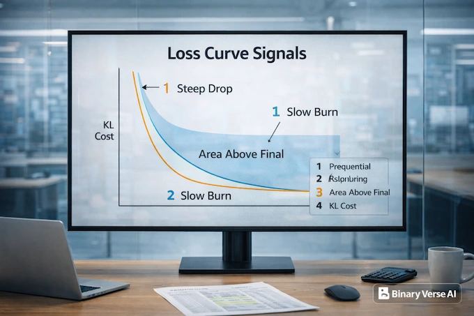
4.1 Prequential Coding: Area Under The Loss Curve
Prequential coding is the easy entry point. You train normally, and treat the loss curve like a bill. The part of the curve above the final loss is a proxy for learned structure, and the final loss is the residual unpredictability. The paper explicitly offers “area under the loss curve above the final loss” as a simple heuristic.
This also reframes loss-curve interpretation. In their cellular automaton experiments, rule 54 shows loss that decreases slowly while “much epiplexity is produced,” while rule 30 yields maximal time-bounded entropy but no epiplexity.
4.2 Requential Coding: Cumulative KL Divergence Between Teacher And Student
If prequential is your quick estimate, requential is the more rigorous accountant. It uses cumulative KL divergence between teacher and student models as the coding cost.
The catch is compute. Requential coding is typically 2× to 10× slower than prequential coding. Empirically, both methods often rank datasets similarly even if the absolute numbers differ.
Epiplexity Measurement Methods: Quick Comparison
Fits the content area. Wraps text, no layout jitter.
| Measurement | What You Compute | What It Estimates | Pros | Cons |
|---|---|---|---|---|
| Prequential | Training loss curve | A proxy for Epiplexity via “area above final loss” | Cheap, uses standard training | Heuristic split of structure vs noise |
| Requential | KL gaps between teacher and student over training | A more rigorous code length for learning | Principled, closer to theory | Slower, more moving parts |
| Final loss only | One number | Mostly time-bounded entropy | Easy to compare | Blinds you to learned structure |
| Downstream eval | Task metrics | Usefulness, not information | Directly relevant | Task-dependent, expensive |
5. Practical Applications: Using Epiplexity For LLM Optimization
Now the part that pays rent. If training is an information extraction pipeline, Epiplexity becomes a metric you can optimize, not as a replacement for loss, but as a missing axis.
The paper makes a pointed framing: MDL is a criterion for model selection on a fixed dataset, while epiplexity is its dual, a criterion for data selection under a fixed compute budget.
A practical workflow for an LLM Optimizer looks like this:
- Sample candidate slices of data (domains, sources, transformations).
- Train small proxy models under a fixed budget.
- Measure epiplexity proxies from training dynamics, not just final loss.
- Keep data that yields high Epiplexity per unit compute, downweight “hard but hollow” junk like hashes and IDs.
This is how you cut AI Training Cost without turning your model into a fragile benchmark chaser.
6. Reducing AI Training Cost With Better Data Selection
Compute is expensive, and it’s getting expensive in the ways that hurt most. GPUs are scarce, energy is real, and a big run is a logistics project, not a weekend script. So the question becomes brutally practical: which tokens are buying reusable capability, and which tokens are just paying rent on randomness?
A good heuristic is to stop asking “Which dataset has lower loss?” and start asking “Which dataset gives me more structure per unit compute?” Favor data where progress comes from learning compact rules, not from memorizing long tails of identifiers. Be suspicious of corpora that are prediction-hard for boring reasons, logs, UUIDs, file paths, random configuration fields. They spike loss, they inflate AI Training Cost, and they rarely build durable skills.
In a mature pipeline, this becomes a loop. Run small proxy trainings, compare loss-curve shape plus your epiplexity proxy, then shift budget toward slices that keep paying back on downstream transfer. That’s LLM Optimization with a finance brain.
7. The Role Of Epiplexity In Synthetic Data Quality
Synthetic data is often pitched as “more data.” The better question is whether it forces the model to learn internal programs it would not otherwise learn.
The paper calls out the tension directly: classical ideas like the data processing inequality make synthetic data look useless, while practice shows it can help. The epiplexity lens resolves it. Deterministic transformations can increase the structural content visible to a bounded learner, even if the generating process is simple.
So Synthetic Data Quality is less “does it look real,” and more “does it create learning pressure for better internal algorithms.” Done well, it boosts Epiplexity and shows up as broader capability.
8. Epiplexity And Out-Of-Distribution Generalization
The paper doesn’t just define terms, it measures them across modalities and links them to downstream behavior.
They estimate epiplexity and time-bounded entropy for OpenWebText, chess, and CIFAR-5M. OpenWebText carries the most epiplexity, chess follows, and CIFAR-5M has the least, with over 99% of its information being random at the pixel level.
They also report that a data selection strategy (ADO) selects data with higher epiplexity, matching improved downstream performance and out-of-distribution perplexity on other corpora.
One important caveat is explicit: Epiplexity measures information extracted, not whether it matches your favorite benchmark. Still, as a debugging tool for LLM Optimization, it’s hard to beat.
9. Conclusion: The Future Of Data-Centric AI
We’ve been living with a mismatch. We talk about entropy, loss, and likelihood like they are the whole story, then we build systems where the real product is the learned internal program.
Epiplexity names the missing part: the structural information your bounded training run can distill into weights. Optimize for that, and you get models that generalize because they have something reusable inside them, not just a big pile of memorized coincidences.
If you run training pipelines, take this as an invitation to upgrade your instrumentation. Plot loss, sure. Then start asking which data slices buy structure, which ones buy noise, and what you’re spending per bit of Epiplexity.
Try it on your corpora this week. Compare domains. Compare orderings. Compare “natural” data to your synthetic pipelines. Then publish what you learn, or send it to me, I love a good mysterious loss curve.
What is Epiplexity in machine learning?
Epiplexity is a measure of how much learnable structure a model can extract from data under a fixed compute budget. It separates reusable patterns from randomness that stays unpredictable.
How is Epiplexity different from Shannon Entropy?
Shannon Entropy measures randomness in the data distribution. Epiplexity measures the structure a bounded learner can actually compress into its weights, which is why high-entropy junk like hashes can be unhelpful for learning.
How do you measure Epiplexity from a loss curve?
A practical proxy is prequential coding, which treats the “area under the loss curve above the final loss” as a rough estimate of learned structure. A more rigorous method uses teacher-student training and cumulative KL costs (requential coding).
How does Epiplexity help with data selection for language models?
Epiplexity helps you prioritize data that forces models to learn transferable structure, not just chase lower loss. That makes it useful for Data Selection for Language Models and for filtering “hard but hollow” tokens that inflate training without improving generalization.
Can Epiplexity reduce AI training cost?
Yes. If you select higher-Epiplexity data, models often learn reusable abstractions sooner, which can lower the compute needed to reach a target capability level. In practice, this is an LLM Optimization lever that targets AI Training Cost directly.