
Imagine a telephone game where every player hears one of four colors and passes a noisy copy to several children. You see every color in the last row. As that row gets farther away, can you still tell what the first player heard? For the ferromagnetic four-state Potts model, OpenAI’s proof locates the exact cutoff on regular and Poisson branching trees. If measures branching and measures the signal retained by one transmission, root information survives precisely when . At equality, the linear signal budget balances exactly, but a cubic loss makes the evidence fade.
Table of Contents
1. What Is the Potts Model?
The -state Potts model assigns one of discrete spins to each vertex of a graph. Ferromagnetic interactions favor neighbors with matching spins. With two labels, this is the Ising model after reparameterizing the interaction.
On a tree, each child samples from a distribution that favors its parent’s color. This turns a question about the influence of a distant boundary into a question about inference from noisy copies.
2. The Four-Color Telephone Tree and the Reconstruction Problem
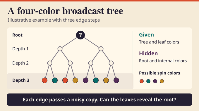
A simple way to implement the channel is to copy the parent with probability and otherwise draw a color uniformly, allowing the draw to match the parent by chance. For colors , with the parent’s color and the child’s, the transition law is
For , a red parent produces a red child with probability and each other color with probability . On a tree with two children per vertex, suppose you observe two red children. By Bayes’ rule, the probability of a red root becomes . With one red and one blue child, red and blue instead tie at each.
At depth , the observer sees the colors exactly edges from the root, along with the tree. Random guessing succeeds one quarter of the time. To express what the full observation tells us, the paper measures the expected total variation distance between the root’s posterior and the uniform prior. That distance is half the sum of the four absolute probability shifts. If it tends to zero, the advantage of even the best root guess also tends to zero.
3. The Kesten–Stigum Threshold and the Longstanding Puzzle
The channel has eigenvalue one on constant functions and eigenvalue on every mean-zero color contrast. For example, give red score one, blue score minus one and the other colors zero. The expected score after a transmission is times the parent’s score. A second-moment calculation therefore picks up for signal strength and a factor of for branching. Above , the classical Kesten–Stigum direction gives reconstruction.
The reverse direction has to bound the entire posterior. A linear calculation predicts what happens to weak signals, while the process starts with an exactly observed spin at depth zero. Combining several weak or strong observations can produce effects invisible to a calculation that tracks individual color contrasts.
The binary symmetric case was already understood, and Allan Sly showed that the spectral criterion can fail for larger Potts alphabets, including ferromagnetic models with at least five colors at sufficiently large degree. Elchanan Mossel, Sly and Youngtak Sohn proved four-state nonreconstruction up to and including the critical point in a sufficiently large mean-degree regime. The paper’s new target is the full range of branching parameters in the two specified families.
4. What OpenAI’s New Proof Establishes
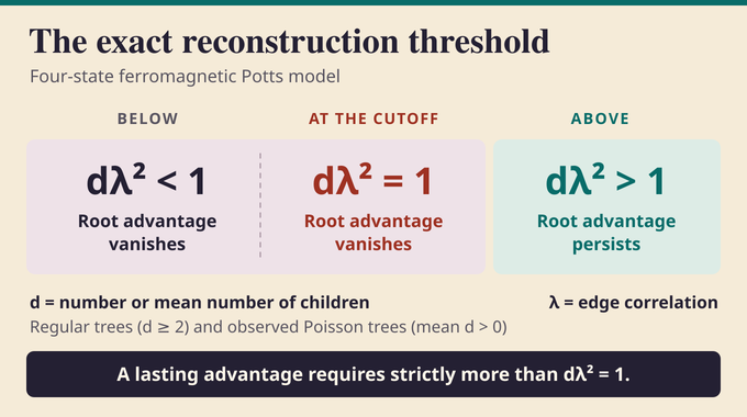
Theorem 1.1 of the October 5, 2026 manuscript gives nonreconstruction whenever and , for every regular -ary tree with integer and every Poisson Galton–Watson tree of real mean . Here counts children or their mean. Paired with the known supercritical result, it makes the threshold exact in both families.
In the Poisson model, the tree is sampled independently of the spins, and the entire unlabelled tree is available to the observer. The expectation includes extinct trees. When level is empty, its observation contains no colors and the tree alone leaves the root uniform. Above threshold, the known reconstruction result applies on survival, which has positive probability in the supercritical range, and so yields a positive advantage after averaging over all trees.
5. The Complete Proof Strategy in Six Stages
OpenAI attributes the release’s results to an internal frontier model. The sequence below reconstructs the manuscript’s argument from its mathematical dependencies. The supplied sources leave open how the model arrived at the particular polynomial.
- Replace the boundary with four probabilities. Each observed boundary induces a posterior over the root colors. Track how those posteriors vary across observations.
- Measure the departure from uniform. Squared distance from the uniform distribution contracts exactly across one edge. Its decay would settle reconstruction.
- Account for how branches agree. Multiply color-by-color evidence and normalize it. The normalization also reweights which observation pairs occur, so the proof must control the update and its averaging together.
- Keep one more statistic. A degree-six polynomial defines a constraint on the distribution of posteriors. The constraint starts out true and remains true after an edge, a branch merger or an observed mixture.
- Find a loss at each branching step. Inside that class of posterior laws, the first two branches yield a strict saving in expected information. At criticality, that saving rules out a positive limit.
- Certify the inequalities on whole regions. Use symmetry, exact coefficients and a finite subdivision of two probability simplices to prove the needed signs. The certificates apply to every allowable posterior pair, including those far from uniform.
6. Measuring Information in Posterior Probability Distributions
The posterior has four nonnegative coordinates that sum to one. Its probability simplex therefore has three independent dimensions. Write for the uniform point. The paper’s quadratic information is
It is zero at and three at a vertex where one color is certain. Across an edge, a posterior about the child becomes about the parent. Every centered coordinate is multiplied by , so for each posterior, and the same relation holds in expectation.
For example, has . Passing the evidence through another edge with gives and . The expected value of gives depth-wise progress. Controlling a merger takes more because the size of a deviation alone leaves out which colors the two observations favor.
7. Why Combining Multiple Branches Is Mathematically Difficult
Two child subtrees produce independent observations conditional on the root color. Marginally, both depend on the same unknown color. For instance, with the two children in the red example, the probability both are red is , while the product of their individual red probabilities is .
Let and be the two individual posteriors about the root after their edge steps. With a uniform prior, their joint posterior is obtained by multiplying corresponding coordinates. Let denote the weight that converts the independent product of the marginal observation laws into the true joint law.
For an expected statistic of , the proof can sample and independently from their respective marginal posterior laws and weight the statistic by . Pairs with have zero weight. Aligned evidence may receive more weight and also move the combined posterior farther from uniform. The denominator and the change of measure explain why a spectral calculation for a single edge leaves the merger unresolved.
8. The Degree-Six Polynomial Behind the Breakthrough
Use three contrasts , and . Permuting the four colors permutes these contrasts and changes an even number of their signs. This makes , and invariant under relabeling. In particular, and capture aspects of the contrasts that their total squared size leaves undetermined.
The manuscript specifies , and as linear combinations of the same nine monomials in , and . The degree-six terms appear in , while and have degree five. The signs of and connect the constraint to each merger. The key condition is for a symmetric posterior law. For an exactly revealed color, . At uniformity it is zero. Individual posteriors can have negative values, such as when two colors each have probability one half. The edge inequality propagates the expectation constraint.
For mergers, the proof averages the weighted update over the 24 possible relative color permutations. Because each marginal law is symmetric, this averaging preserves the desired expectation. The lower bound for the averaged contains the paired terms , where . Under independent marginal sampling, their expectations factor and the result is nonnegative. In the upper bound for , analogous terms with a nonnegative polynomial can be subtracted. The bound also subtracts . If both branches have mean information , Jensen’s inequality turns this last term into a saving of at least .
9. The Cubic Correction That Forces Information to Disappear
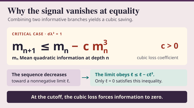
Let be the mean of for the depth- experiment on the ordered tree truncated at that depth. Each branch supplies . Use the saving on the first two branches when they exist, then add at most for each further branch. An observed offspring count is independent of the root, so averaging these bounds over preserves the constraint and gives
For regular branching the probability is one. For Poisson branching it is , positive for every . At the first transmission erases all information. Below threshold, dropping the cubic term already gives geometric decay. At equality, decreases toward a nonnegative limit . The inequality forces , hence . Above threshold, reconstruction comes from the separate Kesten–Stigum result.
The rest of an ordered tree below depth adds no spin information once its truncation is known. Forgetting the ordering can only reduce the expected total variation distance, by convexity. The paper bounds the resulting advantage by . This even covers the noiseless Poisson case , where a nonempty level reveals the root perfectly but has probability tending to zero.
10. Inside the Computer-Assisted Mathematical Proof
The verifier sorts each posterior’s coordinates using color symmetry. The sorted vectors form a simplex. In barycentric coordinates, the proof writes polynomials in homogeneous form by multiplying lower-degree terms by powers of the sum of the coordinates, which equals one. Every monomial is nonnegative there. If all coefficients are nonnegative, the polynomial is nonnegative throughout the region.
The two merger inequalities contain denominators from Bayes’ rule. Type T bounds each inverse power of the normalizer from below using a fifth-degree Taylor polynomial about one. The sixth-order remainder is nonnegative, and the proof first shifts the numerator so multiplication preserves the inequality. Type P interpolates each rational term on a grid with 20 lattice nodes in each simplex. It subtracts an explicit correction certified by coefficient signs after clearing the positive denominator. The checked remainder guarantees the bound between grid points as well. The weighted terms extend continuously by zero where the normalizer vanishes.
When neither test accepts a cell, the verifier splits one simplex at an edge midpoint and checks both children, whose union covers the parent. The manuscript reports the following exact traversal totals.
Appendix A gives C++ and Python verifiers. The reproduction notes distinguish rerunning the full traversals from checking the retained traversal records. Exact arithmetic settles the polynomial signs, while the manuscript supplies the probabilistic argument. The linked Lean scope document covers supercritical reconstruction for a three-state channel. This four-state theorem is established by the manuscript’s computer-assisted argument.
11. Why the Four-State Reconstruction Threshold Matters
This Potts model phase transition identifies when distant leaf evidence can retain a lasting statistical advantage about the root. In statistical mechanics, it isolates a transition in what the boundary reveals about a hidden spin. Other notions of ordering, and graphs with cycles, pose separate mathematical questions. A percolation threshold, for example, asks when an infinite connected cluster can exist. The observable here is the information in the posterior of a single hidden color.
The ferromagnetic assumption matters. Four-state antiferromagnetic examples can reconstruct below the Kesten–Stigum threshold, and the theorem treats regular and Poisson offspring. A natural question is which other offspring distributions admit a comparable threshold proof and whether their branch mergers preserve a useful polynomial constraint. The cubic bound establishes disappearance of information at the threshold. Pinning down the exact rate at which the optimal guessing advantage vanishes is a finer question.
At exact linear balance in the four-state Potts model, the loss from combining branches survives averaging and compounds with depth. Follow Binary Verse AI for more research explainers that work from the theorem back to the idea that makes the proof succeed.
What is the Potts model?
The Potts model assigns each vertex of a graph one of several discrete spin states. In the ferromagnetic version, neighbors favor matching states. In the paper’s tree broadcast model, each child receives a noisy copy of its parent’s state.
What is the difference between the Potts model and the Ising model?
The Ising model has two spin states. The -state Potts model allows states and reduces to the Ising model at after reparameterizing the coupling. OpenAI’s paper studies the ferromagnetic case with .
What is the Kesten–Stigum threshold for the Potts model?
The Kesten–Stigum threshold is , where is the number of children or mean offspring count and measures the correlation transmitted across an edge. For the two four-state ferromagnetic tree models in the paper, reconstruction is possible exactly when .
What did OpenAI prove about the four-state Potts model?
OpenAI proved nonreconstruction for in the ferromagnetic model on every regular -ary tree with integer and every observed Poisson Galton–Watson tree with mean . The Poisson result averages over all trees, including those that die out.
What happens exactly at the reconstruction threshold?
The root posterior converges to the uniform prior in expected total variation as depth grows. The linear coefficient in the quadratic information bound equals one, and a strictly negative cubic correction when information is positive forces its mean to zero.
Is OpenAI’s Potts model proof formally verified?
The four-state result is established by a computer-assisted proof. The paper supplies the probabilistic argument and exact-arithmetic certificates checked by C++ and Python programs. The associated Lean scope document describes a formalization of above-threshold reconstruction for the related three-state channel.