
The Standard Model’s weak interactions distinguish left-handed particles from right-handed ones. Put those fermions on a spacetime grid, and that distinction becomes a problem for the path integral. In his preprint, physicist Nathaniel Craig constructs a gauge-invariant fermion measure for four-dimensional chiral gauge theory at finite lattice spacing, in a class that includes the Standard Model’s fermion content. Craig proposed the refinement strategy, and GPT-6 Astra took the lead in developing the detailed proof through iterations with Craig and outside experts. The result removes a longstanding obstacle to a candidate nonperturbative Standard Model on a finite lattice. The interacting continuum theory remains open.
Table of Contents
1. What Is a Chiral Gauge Theory, and Why Is the Standard Model Difficult to Define?
Chirality separates the components of a spinor according to whether the chirality matrix has eigenvalue or . These are the left-handed and right-handed components. A chiral gauge theory assigns them different gauge transformations. For example, the left-handed electron belongs to a weak doublet with the electron neutrino, while the right-handed electron is a weak singlet. Gauge invariance requires the path integral to respect local changes of gauge frame, including in the rule used to integrate over fermions.
Lattice QCD can treat left- and right-handed quark components in the same color representation. The weak sector of the Standard Model requires a regulator that preserves the difference in gauge charges. The paper works at finite cutoff, meaning the original lattice spacing stays positive while the path integral is defined. This lets the construction address gauge fields throughout the admissible domain without a power series in the gauge coupling.
| Item | Result |
|---|---|
| Setting | Finite periodic four-dimensional Euclidean lattice with sufficiently small plaquettes. |
| Main theorem | Smooth gauge-invariant overlap fermion measure for in . |
| Local guarantee | Exponential locality and the exact lattice anomaly equation. |
| Global guarantee | Matching determinant phases on every closed admissible loop. |
| Standard Model scope | All four global gauge groups, with one copy of the restricted measure per generation. |
2. Fermion Doubling and the Nielsen–Ninomiya Theorem
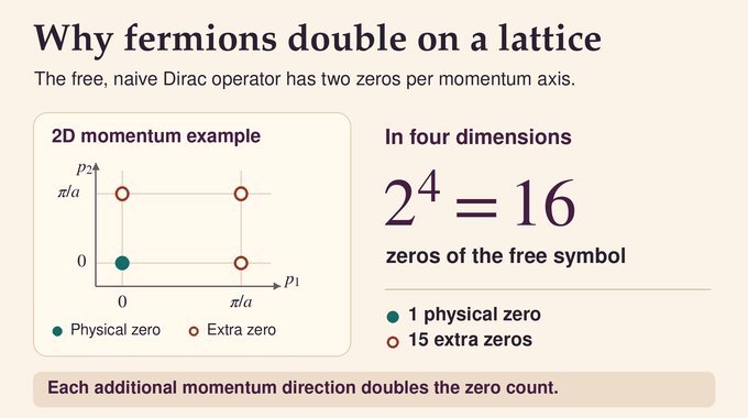
A symmetric lattice derivative replaces momentum in direction by , where is the lattice spacing. On the periodic momentum domain, each component vanishes at both and , with identified with . The four-dimensional free symbol therefore has 16 zeros, one at the desired origin and 15 extra ones. For instance, expanding about gives a linear zero again, with the sign of the first momentum component reversed. This momentum-space count describes the free symbol, while the momenta sampled on a particular finite torus depend on its periods and boundary conditions.
The Nielsen–Ninomiya theorem gives the general obstruction under translation invariance and appropriate locality and regularity assumptions. A lattice Dirac operator with the desired continuum behavior and conventional chirality, , cannot also eliminate the unwanted species under those assumptions.
3. What Overlap Fermions and the Ginsparg–Wilson Relation Already Solved
The Wilson operator adds a momentum-dependent scalar term. In the convention used in the paper, its free form is
Here are Euclidean gamma matrices. The Wilson term contributes for each momentum component at , lifting the extra zeros and breaking conventional chiral symmetry. Gauge links enter the interacting operator through covariant shifts. Define and the overlap operator . The Hermitian operator has a gap on sufficiently admissible fields, where each elementary plaquette is close to the identity. Its sign replaces each eigenvalue by its sign and preserves its eigenspace.
This Ginsparg–Wilson relation gives an exact modified chiral symmetry at finite spacing. With , the fermions and independent antifermions use different projectors.
Since , the fermion projector selects the positive spectrum of . The fermion satisfies , and the antifermion satisfies . The overlap operator has its physical free zero at the origin and takes the value at the naive doubler momenta.
4. Why the Fermion Measure Still Needed a Gauge-Invariant Phase
Write the gauge links collectively as . The fermion subspace selected by depends on , while the antifermion reference space stays fixed. Expand in a local orthonormal basis , with independent Grassmann coefficients . A unitary basis change introduces a determinant phase in the product of Grassmann differentials. The measure needs a compensating phase multiplying that product and the fixed antifermion differential product.
A choice at one field leaves open how the phase varies from field to field. Craig uses Lüscher’s measure term , a one-form that assigns a real number to an infinitesimal link variation. Its coefficients define the measure current on the original links. The current must compensate the overlap operator’s gauge variation, decay in its sensitivity to distant links, and produce globally consistent phases as the allowed subspace changes.
5. Lüscher’s Earlier Construction and the Nonabelian Obstruction
Lüscher’s abelian construction uses the linearity of the abelian field strength in the gauge potential. Scaling the potential in the interpolation scales its curvature as well. On a torus, magnetic flux, Wilson lines, and finite-volume corrections require additional work. For anomaly-free nonabelian theories, Lüscher also developed a measure to all orders in perturbation theory. Nonperturbative constructions covered specific cases, including real representations and an electroweak construction in the sector of zero hypercharge magnetic flux on sufficiently large lattices.
For a nonabelian connection , scaling it by gives curvature
The linear and quadratic terms can nearly cancel at and lose that cancellation at intermediate values. A small endpoint field strength therefore gives no guarantee that the interpolation stays within the plaquette bound. Craig’s construction instead takes comparisons across lattice spacings.
6. Theorem 4.1 and the Chiral Gauge Theory Measure
On a finite periodic four-dimensional Euclidean lattice with the prescribed periodic or antiperiodic fermion boundary signs, Theorem 4.1 treats the overlap operator for with left-handed fermions in . The is the second exterior power of the fundamental representation. The is the conjugate of the fundamental, a separate multiplet whose contribution is essential for anomaly cancellation.
Admissibility requires for every elementary plaquette , where is the ordered product around the plaquette and the norm is the fundamental-representation operator norm. For a sufficiently small positive threshold , the current is smooth and gauge covariant, satisfies the exact lattice anomaly equation, and obeys full integrability on every closed admissible loop. Its exponential locality bounds apply at each fixed derivative order. The threshold and positive decay rate are independent of the volume, component, and derivative order, while bound constants can depend on the order. The current transforms as an axial vector under the corresponding lattice rotations and reflections. Its charge-conjugation law relates currents in the original and conjugate representations. Reconstruction yields a gauge-invariant fermion measure on every nonempty admissible component, with one free constant phase per component for this current.
7. Reconstructing a Connection and Refining the Lattice
Craig reconstructs a smooth connection on the continuous four-torus from the original link transports. Locally, weighted transports between nearby lattice vertices produce a matrix close to a rank-five projection. Its five-dimensional spectral subspace supplies the color space at each point. Projecting derivatives into these spaces and removing the trace part gives an connection. Local frames let the construction work on a gauge bundle that may be nontrivial.
The original field is level zero. At positive levels, the same connection provides the edge transports on auxiliary lattices with spacings in original lattice units. Small plaquettes on these lattices approach the identity quadratically in the spacing. This refinement is part of the definition of the measure for the original operator. The physical cutoff stays fixed throughout.
8. Comparing Chiral Projectors to Construct the Measure Current
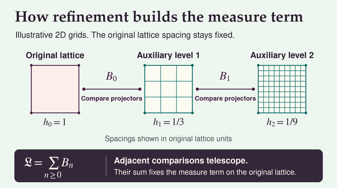
Each coarse site has children on the next lattice. In transported color bases, the embedding copies the spinor to each child with a factor of , preserving its site-sum norm because . The coarse Hermitian Wilson operator acts on this embedded subspace. On the extra fine states it is extended by , so their determinants cancel against the corresponding antifermion reference factors.
The interpolation runs from the fine Hermitian operator to the extended coarse one. A uniform spectral gap keeps its positive-spectrum projector smooth for the entire comparison, with the interpolation parameter. For a variation of the original links, the comparison integrates a mixed component of projector curvature.
The capitalized trace includes all states of the comparison space. The exterior derivative of is the coarse curvature minus the fine curvature, both evaluated on the original field variations. Thus the intermediate curvatures cancel in a sum. The same comparisons multiply ratios of coarse to fine determinant phases, so the intermediate phases cancel as well. The original field stays at the coarse end of the first comparison, so the term left there is exactly the one that enters the reconstruction conditions. The resulting candidate measure term is
9. How Anomaly Cancellation Gives Convergence and Exponential Locality
The complete multiplet has zero cubic gauge anomaly. Craig obtains this from the character difference , where acts on the five fundamental colors on the right. For , each of the five matrix directions contributes at least one power of , so the determinant is . The cubic traces in the two representations thus coincide, and complex conjugation gives them opposite signs. Expanding in several generator directions gives the corresponding mixed cubic identities. The proof also uses equality between the ordered color traces in and through four Lie-algebra factors. Spin conjugation gives the opposite sign for the relevant real contributions, so those terms drop out of the full representation sum.
The gap supports exponentially decaying polynomial expansions of the projector. In a local radial frame, a background transport insertion supplies two powers of the fine spacing. For the current, one prescribed link variation can contribute without a small-spacing factor. Four further factors supply eight powers of spacing before the sum over fine sites, whose count scales as at fixed original volume. The locality proof controls that counting in neighborhoods of each original link, including at every fixed order of original-link derivatives.
| Quantity | Bound | Role |
|---|---|---|
| First comparison | Finite contribution from the original lattice. | |
| Later comparisons | Summable for . | |
| Pulled-back curvature | Vanishes as the auxiliary lattice is refined. |
Bounds use exponential locality norms at any fixed derivative order . The constants may depend on .
For comparison, the curvature contains two prescribed link variations. Three extra background factors give six powers of spacing before the site sum, leaving two powers. The curvature remainder therefore tends to zero, so , the original projector curvature. Evaluated on an infinitesimal gauge transformation, each comparison instead gives the coarse anomaly minus the fine anomaly. The finest remainder vanishes at fixed original field, volume, and gauge parameter. The resulting link current obeys
Here is the backward covariant difference and is the lattice gauge anomaly density at site in generator direction . A nonzero density at finite cutoff is consistent with this equation. Its contribution to the gauge variation is canceled by the measure.
10. Global Integrability and Path Independence
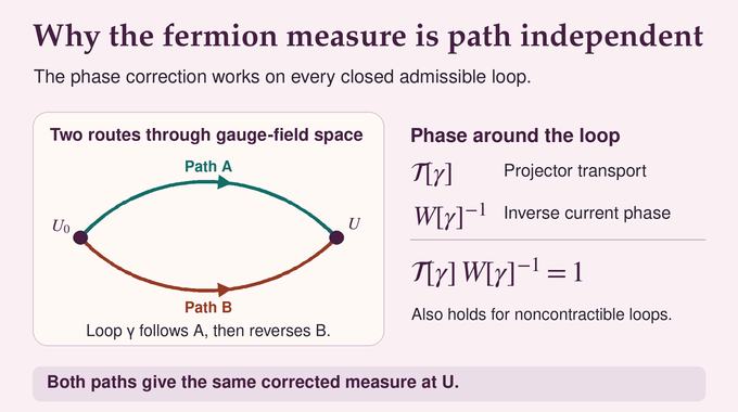
A curvature identity controls infinitesimal loops. A closed loop that cannot be shrunk inside the admissible domain can still carry a phase, so the proof also needs
Here is the determinant phase from transporting the original chiral subspace around the loop relative to the antifermion reference. By telescoping, the only phase to control is the one on the finest sampled lattice.
For a fixed loop, the reconstructed bundle lives over the four-torus times the loop circle. Two globally defined orthonormal color sections leave a rank-three complement, enabling a comparison with an auxiliary connection on the same bundle. The fermion representation restricts there to two triplets, two antitriplets, and three singlets. In combination with spin conjugation, the color pairing makes the auxiliary covariant transport eigenvalues come in conjugate pairs, fixing its determinant phase to . The cylinder interpolates between two connections on the same bundle. Its fine samples become admissible as the spacing shrinks. Two corrections, from curvature on the cylinder and from removing the auxiliary color transport, vanish in that limit.
The ordinary fine-lattice phase therefore tends to one for each closed loop, including noncontractible ones. Starting at a reference measure, multiply projector transport by the inverse phase from the current. Their phases cancel on every closed loop, yielding the same measure along any path to a given field. This argument also covers overlap zero modes.
11. From SU(5) to the Four Standard Model Gauge Groups
The paper treats all four global forms , for . Map an element of the product group to the block diagonal matrix in . The product group map has kernel . Its induced map on is injective only for , so the paper tests admissibility in a faithful representation of each actual quotient. This catches plaquettes that the image alone could miss.
The restriction of gives one generation in left-handed notation, which describes right-handed particles using their left-handed charge conjugates. For example, the includes the quark doublet with integer hypercharge . Pulling the measure back along the link map preserves locality and the phase identities. Three independent copies give the three generations. The construction uses the Standard Model gauge variables and includes nonliftable bundles wherever their admissible lattice components are nonempty.
12. Lean Verification, Physical Implications, and Open Problems
The paper reports that all 16 Lean 4 modules of the mathematical companion compiled. A separate kernel replay and axiom checks accepted the formal proofs with standard foundational axioms and no unproved placeholders. The development covers the construction and its four Standard Model restrictions, including the current’s locality, anomaly, and integrability properties under the encoded assumptions. The manuscript also reports a two-dimensional check against directly evaluated gauge responses and determinant phases. A second construction, starting directly from a reference state and averaging phase corrections, agrees up to exponentially local counterterms.
The chiral gauge theory result gives a consistent finite-cutoff fermion measure in the specified domain. Appendices give polynomial approximations and classical continuum estimates for smooth backgrounds. Efficient numerical implementation and a physical choice of phases across disconnected components remain open. So does reflection positivity compatible with admissibility, a condition used to recover a Hilbert space with a positive inner product from Euclidean correlators. Establishing the interacting continuum theory is a separate problem. This is the distinction that matters when reading the result as progress toward Standard Model lattice gauge theory. Follow Binary Verse AI for research explainers on what finite-cutoff constructions and continuum existence proofs each establish.
What is a chiral gauge theory, and how does chirality differ from helicity?
A chiral gauge theory couples left- and right-handed fermion components differently to gauge fields. Chirality is defined by the eigenvalues of the γ₅ operator. Helicity is the projection of spin along momentum. For a massless particle they correspond in the usual particle convention, while for a massive particle helicity can change under a boost. The Standard Model’s weak interactions distinguish chirality.
Why does fermion doubling obstruct a lattice formulation of the Standard Model?
A naive symmetric lattice derivative introduces unwanted extra species. Under its locality, regularity, and translation-invariance assumptions, the Nielsen–Ninomiya theorem rules out a lattice Dirac operator that has the desired continuum behavior, avoids extra species, and preserves conventional chirality. Overlap fermions evade the obstruction through a modified lattice chirality relation.
Why didn’t overlap fermions and Lüscher’s earlier work already solve the problem?
Overlap fermions provide exact modified lattice chiral symmetry. Their fermion integration subspace depends on the gauge field, so a consistent measure phase still has to be chosen. Lüscher constructed nonperturbative abelian measures and developed a nonabelian construction to all orders in perturbation theory. Craig’s result supplies a nonperturbative measure for the specified class of nonabelian chiral theories.
What is the central mathematical innovation in Craig’s Astra-assisted proof?
The proof compares chiral projectors on successively finer auxiliary lattices while keeping the original physical operator fixed. The comparisons give a convergent series for the measure current. Anomaly cancellation supplies the locality estimates, and a separate global argument matches the phases around all closed admissible loops. Together these results enable reconstruction of the gauge-invariant measure.
How does gauge anomaly cancellation make the construction possible?
The cubic gauge anomaly cancels between the 10-dimensional antisymmetric representation and the conjugate fundamental of SU(5). The proof uses the corresponding ordered color-trace identities to cancel low-order terms in the refinement estimates. This makes the series converge with exponential locality and allows the current to satisfy the exact lattice anomaly equation.
Has Craig’s Astra-assisted chiral gauge theory proof been formally verified in Lean?
The paper reports that all 16 Lean 4 modules for the mathematical companion compiled, with separate kernel replay and axiom checks and no unproved placeholders. The formal development covers the SU(5) construction and its restriction to the four Standard Model gauge groups. The checks establish the encoded mathematical results under their recorded assumptions.
Does the proof mean the complete Standard Model can now be simulated nonperturbatively?
The result gives a candidate nonperturbative lattice definition by constructing a gauge-invariant chiral fermion measure at finite cutoff. Practical simulation of the complete Standard Model, reflection positivity compatible with admissibility, and construction of the interacting continuum theory remain open.