

A stack of exact Gaussian equations can pin down an unknown vector after just as many measurements as it has coordinates. Put those same equations through a learner that can read each pair only once and retain at most a fixed multiple of the dimension squared in bits, and the precision changes what it needs. OpenAI’s September 2026 preprint proves a memory sample tradeoff for noiseless Gaussian regression. In sufficiently high dimension, achieving angular error at most with probability at least two thirds requires a sample horizon of at least a constant times , where is the dimension. Each label can carry arbitrarily fine information. The proof measures how much of that information can influence the estimate after repeated finite-state updates.
Table of Contents
1. What Is the Memory Sample Tradeoff in Noiseless Gaussian Regression?
| Item | Study Setup |
|---|---|
| Signal | Uniform random unit vector in dimension |
| Observations | Independent Gaussian rows and exact inner products |
| Persistent Memory | At most bits for fixed finite |
| Accuracy | Angular error at most , with probability at least two thirds |
| Sample Horizon | At least in sufficiently high dimension |
An exact label supplies a linear constraint on the signal. After the learner reads that constraint, any influence it has on later computation must pass through the persistent state or the decision to stop. Success means recovering the direction of the signal on the unit sphere to a prescribed angular tolerance.
The theorem concerns the deterministic deadline by which the learner must stop. A learner may end some runs earlier. This matters when reading the result as a statement about Gaussian regression sample complexity. The lower bound applies to the allowed horizon of any learner meeting the success guarantee.
2. Why Exact Gaussian Measurements Normally Determine the Signal
Let be the unknown unit vector. Each independent standard Gaussian row has covariance , the identity matrix. The observation model is
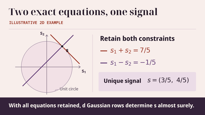
Stack rows into a square matrix and the labels into a vector . Each new row avoids the span of the preceding rows with probability one, because a proper linear subspace has Gaussian measure zero. Thus is invertible almost surely, and the retained system has the unique solution .
For a small example, take rows and with labels and . Adding and subtracting the two equations recovers the unit vector . These are illustrative rows. In the Gaussian experiment, the independence of the row directions needed to solve the full system holds almost surely. The example shows what a solver needs from both observations. It must preserve enough information to combine their constraints. An exact real entry can require arbitrarily many bits to retain.
3. The Finite-Memory Learner and What It Can Remember
A learner with bits has at most persistent states at each index. Its rules may depend on dimension, accuracy and sample index. It can examine the entire current pair, use fresh randomness and compute without a time bound before retaining its next state. The initial state and any shared seed that selects the rules are jointly independent of the signal and all Gaussian rows.
The learner reads the stream in order, can stop at index zero, and must stop by a prescribed finite horizon . Given the shared seed, the output rule uses the terminal state, the stopping index and fresh randomness to produce a unit vector. The stopping index can itself carry information, so the proof counts distinct stopping times alongside memory states.
The paper also imposes joint measurability on the experiment and requires Borel or reference-measure-completed transition and stopping probabilities at fixed seeds, states and indices. The proof handles completed-measurable rules by replacing them with Borel versions for almost every shared seed, preserving success averaged over the sphere. The model isolates persistent storage as a resource in streaming linear regression and memory-bounded learning.
4. The Main Theorem on Precision and Samples
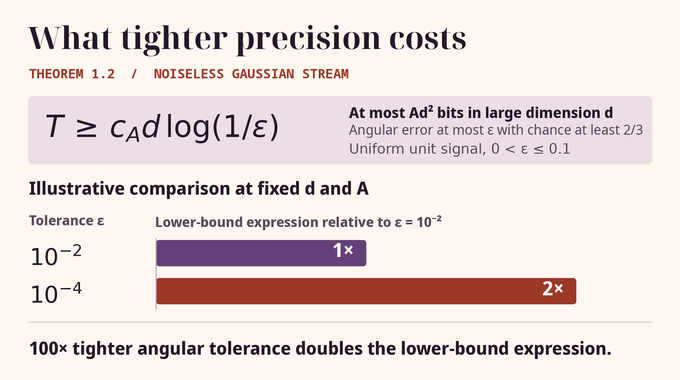
Theorem 1.2 fixes any finite . There are constants and such that for , integer , and , the following implication holds. Draw uniformly from the unit sphere, independently of the rows and the learner’s data-independent randomness. If the unit output meets the guarantee below, the horizon obeys the stated lower bound.
The angle is in radians. The probability averages over the signal, rows and learner randomness. A guarantee of at least two thirds for every fixed signal implies the average guarantee. For , the constant can be absolute once the dimension is sufficiently large for the given memory sequence.
For example, tightening the tolerance from to changes the natural logarithm from to . At fixed dimension and memory cap, that doubles the theorem’s lower-bound expression. The bound leaves the optimal horizon unspecified.
5. What Earlier Noisy Regression Lower Bounds Could Not Establish
In 2019, Vatsal Sharan, Aaron Sidford and Gregory Valiant studied memory-constrained linear regression with the same isotropic Gaussian covariates and independent uniform additive noise of half-width . Their lower bound was at Euclidean tolerance , for memory at most bits and from a sufficiently large constant up to order .
An exact-data learner can generate independent noise inside its current transition and simulate a noisy-data learner with the same state budget. A lower bound for the noisy task leaves open whether a learner could exploit exact labels to use fewer samples. A lower bound for the exact task can carry over to that noisy experiment under the appropriate model and accuracy conversion.
6. Why Exact Observations Break the Usual Posterior-Density Argument
After seeing a raw pair , the compatible signals lie where the unit sphere intersects the hyperplane . This section has zero mass under the original sphere prior, even though it contains the conditional signal almost surely. The raw-data posterior is therefore singular relative to the original spherical measure.
The proof instead fixes a state and index and asks a different question. For each signal , what is the chance of success if the learner starts in that state and receives fresh future rows? Call this probability . Integrating against the original sphere prior weights signals by their future success. This includes states the learner never visits. Defining the continuation this way lets the proof work backward from the output rule without conditioning the prior on past observations.
7. Step One: Measure Successful Signals Using Local Spherical Mass
Let denote uniform probability on the sphere and the closed Euclidean ball of radius centered at a sphere point . The ball cuts out a spherical cap of mass at most . For , one can see this by projecting the cap onto the coordinate plane perpendicular to . Its projected radius is at most and its surface-area factor is at most two. For larger radii, the total mass bound of one suffices.
For a fixed terminal output, successful signals have chord distance at most from that output, because chord distance is at most angular distance. Averaging over the terminal output distribution preserves the resulting global mass bound . Inside any , the successful mass is also at most since . The smaller bound is at most their geometric mean. This initializes the invariant
at . Here controls how concentrated successful mass may be, through an upper bound on the mass inside every test ball. The inequality must hold at every radius so the next step can restrict the measure to any ball and still control its mass on smaller balls.
8. Step Two: Control Exact Gaussian Projections Using Gram Determinants
Fix a destination and restrict its success-weighted measure to . Denote the resulting finite measure by . Write for the Gaussian matrix of a block of rows, reserving for the memory-cap constant. The exact data map is . The proof bounds the density of the joint image measure relative to Gaussian matrix probability times Lebesgue measure on the labels.
The density calculation starts by smoothing the labels with a Gaussian of variance in each coordinate. This is a proof device that is removed in the limit. To bound the th moment of the smoothed density, expand it using copies integrated against . For , the zero-density calculation for the Gaussian label differences is controlled by . Gram–Schmidt writes the determinant as a product of squared distances from each new point to the affine span of the preceding points.
Small distances could make those inverse powers large. The local mass bound controls how much measure can lie in a thin tube around each affine span. For a tube of width around a -dimensional affine span, covering the relevant portion of the tube takes order balls of radius proportional to , with dimension-dependent constants. The resulting mass bound decays like . This decay makes the inverse th moment finite when , which holds for the block lengths and moment order used in the proof. The resulting bounds are uniform as tends to zero. Testing against continuous functions of compact support then gives an density for the exact data.
9. Step Three: Why Projected Ellipsoid Volume Cancels the Density Loss
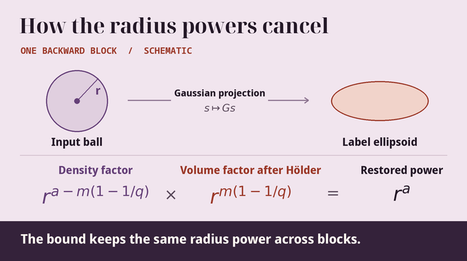
Each destination density has an bound with a factor . All these densities are supported in the same set of matrix–label pairs. For fixed , the label region is the ellipsoid . Almost surely, its semiaxes are times the singular values of , so the label volume scales as . After averaging over , the joint reference measure of the support is at most for an absolute constant .
Hölder’s inequality pairs each density with its routing probability. A second application across destinations collects the routing terms. Their sum of conjugate powers is at most one at any data point, since raising numbers in the unit interval to a power greater than one can only decrease them and the probabilities sum to at most one. The resulting support-volume factor is raised to . Multiplying the radius factors gives
The same radius power returns in the bound before the block, so it can be used again at the preceding boundary. Density control alone would leave the wrong power of .
10. Step Four: How Finite Memory Forces the Backward Sample Bound
A block of observations has at most local stopping indices, including its entrance. Each stopping index contributes up to terminal states. Continuing past the block contributes at most another states. Thus the number of destinations is , even though the block may route using its entire real-valued data.
Hölder across destinations costs a factor in the local mass bound. Taking the th root to update changes this to . With , both and grow proportionally to . Consequently the logarithm of the scale multiplier per block is at most for an absolute constant . The finite state contributes through its logarithmic size, which explains the quadratic memory scale in this argument.
Starting at the last block with , each backward step can multiply the scale by at most a constant for fixed . A ball of radius two centered at any sphere point covers the whole sphere. Average success of at least two thirds forces the initial scale to reach a positive constant. If bounds the scale multiplier and is the block count, then the initial scale is bounded by . To reach constant success, that upper bound must itself be at least a positive constant. Taking logarithms forces to grow at least proportionally to at fine precision. Since all blocks except possibly the last have length , this gives the factor of in the sample bound.
11. Completing the Proof With Constant Accuracy, Kaczmarz, and Limitations
For constant accuracy the proof uses a separate argument. Give the learner every row and label up to the deadline. Reflect the signal across the row span by negating its perpendicular component. The uniform prior is unchanged, and both signals give identical data. If the perpendicular component has norm greater than , the two signals are more than apart. A single estimate cannot be within chord distance of both. The expected squared length in the row span is at most . A Markov bound on that length and the reflected-pair argument give success below two thirds for throughout the stated tolerance range. This supplies the linear floor where the backward estimate alone can be too weak.
The paper uses Kaczmarz as a real-register benchmark. Start from and project the current estimate onto each new measurement hyperplane. For a nonzero row the update is
The correction changes the estimate along the current row by the amount needed to satisfy the new equation. This removes the error component parallel to the fresh row. By isotropy this removes of the squared error in expectation, conditional on the current estimate. After steps, the expected squared error is . Since this is at most , reducing the expected squared error to order takes order steps.
OpenAI’s release announcement describes the broader project. For this manuscript, the Family 140 scope document identifies the main memory–precision theorem and supporting inverse Gram moment, exact projection, regularization and block estimates in Lean. The linked Lean comparator records the selected formal statements. The theorem concerns fresh isotropic Gaussian rows and finite-state, one-pass estimation. Its hypotheses fix the row law and the access pattern, leaving adaptive measurement design and repeated passes outside the result. It leaves open a matching finite-bit algorithm and gives no uniform constant for a memory multiplier that grows with dimension.
The memory sample tradeoff distinguishes the information in an exact observation from what a streaming learner can carry forward. Here the cost of recovering a more precise direction shows up in how many fresh measurements the learner must be allowed to read. Follow Binary Verse AI for more research explainers on time–space tradeoffs, dimension reduction and machine-checked mathematical proofs.
What is a memory-sample tradeoff in machine learning?
A memory-sample tradeoff describes how restrictions on retained information affect the number of observations required for learning. This paper proves such a lower bound for one-pass noiseless Gaussian regression.
Why are d noiseless measurements not always sufficient for linear regression?
With the complete measurement system retained, d independent Gaussian equations determine a d-dimensional signal almost surely. A finite-state streaming learner cannot necessarily preserve all the information needed for this reconstruction.
How does limited memory affect the sample complexity of Gaussian regression?
For every fixed A > 0, memory at most Ad² bits requires a sample horizon of at least cAd log(1/ε) to achieve angular error at most ε with probability at least two thirds in sufficiently high dimension, for 0 < ε ≤ 1/10.
Why does the memory bound involve d² bits?
The proof groups observations into blocks of length proportional to d. Its local-success argument charges memory through a factor governed by M/d². This gives the quadratic scale in the proof and leaves the location of any sharp threshold open.
How is noiseless Gaussian regression different from noisy linear regression?
Noiseless regression uses exact inner-product labels. Earlier bounds for labels with additive noise leave open what can be achieved when the learner receives exact observations.
Does the proof show that the Kaczmarz algorithm achieves the bound with finite memory?
The paper analyzes Kaczmarz with real-valued registers to explain the d log(1/ε) precision scale. A matching algorithm under the finite-bit model remains open in the paper.
Is the memory–sample lower bound formally verified in Lean?
OpenAI’s Family 140 scope document identifies the main lower bound and supporting projection estimates as formalized in Lean. The repository links the comparator statements so readers can examine the scope directly.