
Can a space satisfy the algebraic tests for two dimensions yet still require three? The Wall D2 Problem asks exactly that question about finite cell complexes. OpenAI’s October 6, 2026 manuscript constructs a finite three-dimensional complex satisfying the D(2) conditions but admitting no finite two-dimensional homotopy model. Its fundamental group is infinite. The decisive obstruction combines a character detecting an order-two element with vanishing second twisted homology, a combination the paper proves impossible in finite two dimensions. Here is how the cyclic-cover argument, plus construction and explicit matrix calculation fit together, and where computer verification stops.
Table of Contents
1. What Is Wall’s D(2) Problem?
A CW complex builds a space from cells: points, edges, disks and higher-dimensional pieces attached along their boundaries. “Finite” means finitely many cells, not finitely many points or a finite fundamental group. Wall introduced his dimension conditions in 1965. The unresolved step was whether certain algebraically two-dimensional finite spaces always possess genuinely two-dimensional finite models.
| Feature | What the Manuscript Establishes |
|---|---|
| Research source | A Counterexample to Wall’s D(2) Problem, OpenAI, October 6, 2026. |
| Constructed space | Finite, connected, three-dimensional CW complex. |
| Fundamental group | Infinite, with an element of order exactly two. |
| Negative conclusion | No homotopy equivalence to any finite CW complex of dimension at most two. |
| Verification scope | Written topological proof and partial, conditional community Lean formalization. |
Homotopy equivalence preserves a space’s structure through continuous deformations of maps. It does not require a literal flattening. Two spaces qualify when maps in both directions compose to maps homotopic to their respective identities. The finite-model requirement is essential throughout this argument.
A presentation complex gives a useful mental model: each generator becomes an edge loop, and each relation becomes an attached disk. Three-cells can impose relations among these disks. Wall’s question asks whether the prescribed algebraic vanishings guarantee that those three-cells can be eliminated while preserving the homotopy type.
2. The D(2) Conditions: When Three Dimensions Look Like Two
Write for the fundamental group and for the universal cover, where loops have been unwound. The paper’s initial D(2) formulation requires:
The second condition holds for every finitely generated -module , interpreted as local coefficients. Theorem 1.1 constructs an example satisfying the stronger statement for every such module, without finite generation. Here is the integral group ring, encoding integer combinations of group elements.
The first condition rules out homology above degree two upstairs. The second tests third cohomology using coefficient systems that can change around loops. Neither says the space already has a two-dimensional cell structure. The challenge is geometric realization: can the algebraic disappearance of a dimension be implemented by a homotopy equivalence? No asphericity assumption is imposed.
Checking ordinary third homology alone would be insufficient. The universal cover and the quantifier over coefficient modules retain information about how loops act on cellular chains. The construction must meet those stronger requirements before any obstruction to a two-dimensional model can count as an answer to Wall’s problem.
3. Why Earlier Approaches Could Not Settle Wall’s Problem
Stabilization provides one escape route. Cohen’s result allows sufficiently many two-spheres to be joined to a finite D(2) complex so that the enlarged space has a finite two-dimensional model. As the manuscript recounts, Hambleton bounds the number of added spheres by the number of three-cells. This changes the space, leaving Wall’s original question unanswered.
Group-specific results also gave positive answers. The paper cites Hambleton for finite subgroups of the three-dimensional rotation group and Hofmann–Nicholson for generalized quaternion groups of orders 24 and 32, with order 28 covered through earlier work. These results constrain where a counterexample can occur.
Relation-gap approaches offered candidates, but their negative conclusions depended on unresolved assertions about normal generators versus module generators. The new argument instead supplies a direct obstruction from twisted homology. Its crucial question is whether a character can detect torsion while second twisted homology vanishes.
The distinction between stable and actual realization is particularly instructive. Adding spheres can supply extra two-dimensional homotopy data that enables a realization. One cannot simply subtract those spheres from the resulting model and assume the original space has been realized. The new obstruction applies to the original homotopy type.
4. OpenAI’s Counterexample: Theorem 1.1 Explained
Theorem 1.1 states that a finite connected three-dimensional complex satisfies both D(2) conditions, even with arbitrary coefficient modules, but has no finite homotopy model of dimension at most two. This is the manuscript’s negative answer to the general finite Wall D2 conjecture.
The construction begins with a finite presentation complex, then kills a carefully chosen perfect normal subgroup through a finite plus construction. The resulting quotient group retains detectable torsion. A small twisted boundary matrix proves the required homology vanishing. Finally, a theorem about finite two-dimensional spaces makes those two properties incompatible.
This sequence separates construction from obstruction. Producing a D(2) complex alone would not settle the problem. The proof must also exclude every possible finite two-dimensional replacement, including replacements with entirely different cells. Twisted homology supplies that homotopy-invariant test.
The cell accounting is small enough to follow explicitly. The starting presentation complex has one vertex, five edges and four two-cells. Killing the two normal generators adds two two-cells, followed by two three-cells. Thus the final complex has one, five, six and two cells in successive dimensions, with Euler characteristic zero.
5. Twisted Homology: The New Obstruction to Two-Dimensionality
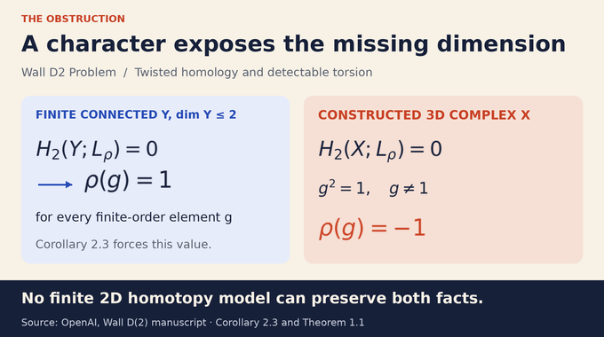
A rank-one complex local system assigns a copy of to each point. Transport around a loop multiplies its coefficient by a nonzero complex number. After choosing a basepoint and basis, this monodromy is a character . “Rank-one” describes the coefficient fiber, not the homology group.
Corollary 2.3 proves that for finite connected of dimension at most two:
Torsion here means an element of finite order in the fundamental group. The conclusion does not forbid torsion itself. It forbids a character with vanishing second twisted homology from detecting that torsion.
For a worked coefficient example, monodromy identifies transport around a loop with a sign reversal. In degree zero, coinvariants impose . Over , this forces . More generally, any nontrivial rank-one monodromy makes zeroth twisted homology vanish. That elementary observation drives the Euler-characteristic argument.
Twisting also changes the second cellular boundary: each traversal of an edge carries the transport factor accumulated along the preceding path. Consequently, two coefficient systems on the same cell structure can have different second homology. The proof selects a particular character whose boundary matrix becomes injective, while its action on torsion remains visible.
6. The Infinite Cyclic Tower: Why the Obstruction Must Hold
Lemma 2.1 establishes persistence under infinite cyclic covers. For finite two-dimensional , the lifted cellular boundary has entries in ], where records the deck transformation. Setting recovers the boundary downstairs. An injective downstairs matrix has a nonzero maximal minor. The corresponding Laurent-polynomial minor is therefore nonzero, proving injectivity upstairs over .
Theorem 2.2 then considers a map from a finite connected simplicial complex with and nontrivial pulled-back monodromy. Its finite image inherits vanishing second twisted homology because, in dimension two, second homology injects from subcomplexes.
Nontrivial monodromy also kills degree-zero homology. Euler characteristic consequently gives , forcing positive ordinary first Betti number and a surjection onto . The map from lifts to that infinite cyclic cover because every homomorphism from its fundamental group to is zero.
Repeat with the lifted image. Equal simplex counts would produce a section of the nontrivial cover, which is impossible. Each image therefore grows strictly while the fixed domain bounds its size:
Here the counting function records nonempty simplices. Keeping one fixed triangulation of the domain makes the contradiction finite and decisive.
There are two distinct uses of finiteness. Each image has finitely many simplices, permitting Euler-characteristic and matrix arguments. The domain supplies a single uniform bound for every stage. The covering spaces themselves are infinite, but the construction retains only the finite image of the lifted map before beginning the next stage.
7. Quillen’s Plus Construction: Building the Finite D(2) Complex
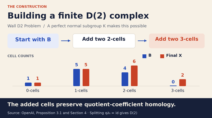
Proposition 3.1 starts with a finite two-dimensional complex and a perfect normal subgroup of , normally generated by finitely many elements. Perfect means ], equivalently that its abelianization vanishes. Finite normal generation is weaker than finite generation as a group.
Attach one two-cell per normal generator, killing , then one three-cell per added two-cell. Suitable attaching maps give a projection onto the new two-cell coordinates satisfying:
This splitting makes the third cellular boundary injective. It also extends every degree-three cochain to degree two, proving third cohomology vanishes for every coefficient module. The relative chain complex is an identity map between free modules in degrees three and two, so it is contractible.
Consequently, homology with any coefficients from the quotient group is preserved. This last property is essential: the twisted calculation can be performed on the simpler presentation complex and transferred intact to the final three-dimensional space.
Why does perfectness permit the needed three-cell attachments? The covering of the original complex corresponding to the killed subgroup has zero first integral homology. The relative homology sequence then supplies two-dimensional classes mapping onto the new cell coordinates. Upstairs, simple connectivity lets the degree-two Hurewicz theorem represent those classes by spheres, providing the attaching maps.
8. The Explicit Group Presentation: Why 15 and 26 Matter
The presentation has generators and four defining relations:
Set , , let be their normal closure in , and put . The matched exponents give and . With , the relations yield:
Write for the images of the two normal generators in . Conjugation gives and . Geometric sums of these relations produce and . The first relation also gives .
Since , both annihilators force . The second module relation then forces . Their conjugates generate the abelianization, so is perfect. The coprime numbers certify that no abelian residue survives, enabling the plus construction.
The geometric sums are doing more than numerical bookkeeping. Conjugation by a normal generator becomes trivial after abelianization, allowing the sums to telescope. Meanwhile, the relevant power relation makes the other action fix the selected generator image. Together these facts turn group relations into the two integer annihilators needed for the final coprime argument.
9. The Character That Detects an Element of Order Two
Choose a primitive cube root , so but . Define the character by:
| Generator | Assigned Value |
|---|---|
The conjugation relations become and . The remaining relations become and . Both normal generators map to one, so the character descends to .
In the quotient, . Yet , so is not the identity and has order exactly two. Separately, sending to one and the other generators to zero defines a surjection . This proves the group is infinite. The example’s finiteness refers solely to its cells.
Both checks matter. A relation saying an element squares to the identity only bounds its order, since the element might itself be trivial. The nontrivial character value excludes that possibility. Conversely, detecting one torsion element says nothing about the size of the whole group. The separate surjection establishes infinitude without any ambiguity.
10. Fox Derivatives: The Matrix Calculation That Completes the Obstruction
To compute the twisted boundary, rewrite the four relations as words equal to the identity. Fox derivatives obey and . Evaluate the group-ring coefficients using the character.
For , the two relevant entries are and . Thus the first row’s second entry is . The second row uses the alternating sum , giving .
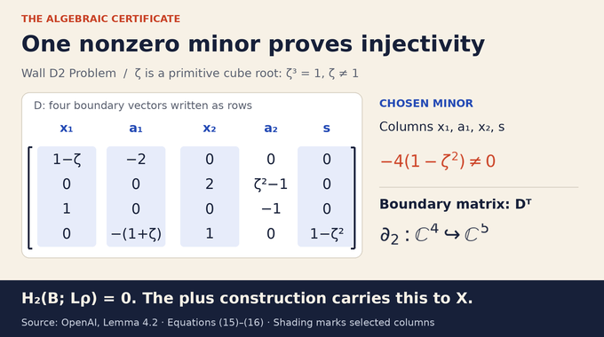
The word gives entries one and minus one. For , the nonzero entries are , one and . In column order , the boundary vectors are rows of:
Selecting columns one, two, three and five gives:
The four rows are independent. With boundary vectors written as rows, the column-vector boundary matrix is , an injective map . Since has no three-cells, . The plus construction transfers this vanishing to .
The selected minor can also be checked without expanding a large determinant. Its last column has only one nonzero entry. Expanding along that column leaves a three-by-three determinant equal to minus four. Multiplication by the remaining entry gives the stated result, which is nonzero because a primitive cube root cannot have square one.
11. The Final Contradiction: What OpenAI’s Proof Establishes and What Remains Open
Assume had a finite two-dimensional homotopy model . Transfer the character across the induced fundamental-group isomorphism. Homotopy invariance preserves zero second twisted homology, but the character still sends an order-two element to minus one. Corollary 2.3 rules this out.
Concretely, the torsion loop extends to a map , because its square is nullhomotopic. The real projective plane has zero first rational Betti number, yet the pulled-back monodromy is nontrivial. This is the forbidden input to the tower theorem.
The manuscript therefore gives a negative answer to the general finite Wall D2 Problem. Its infinite-group example does not settle the restriction to finite fundamental groups. It also supplies no practical-performance benchmark. OpenAI’s mathematics release announcement provides provenance, rather than independent verification of this particular theorem.
The community Lean project’s verification report identifies checked algebraic components, including perfectness, order-two detection and Fox-row independence. Its counterexample theorem remains conditional on named topological assumptions plus_assembly and howie_tower, with an abstract IsAssemblyGroup predicate. The topology and local-coefficient machinery are not fully formalized there. These checks support specific calculations, not a complete machine verification of the written proof.
The conclusion concerns the minimum dimension among finite complexes in the same homotopy type. A complicated cell decomposition alone cannot certify that minimum: many spaces admit simpler decompositions. Here the character and its homology travel across any proposed homotopy equivalence, so the contradiction survives every finite two-dimensional candidate. This explains why a small presentation can settle a broad universal question. Its role is to realize one carefully engineered collection of properties, while the tower theorem supplies the obstruction applying to all possible finite two-dimensional models.
The enduring lesson is that algebraic dimension tests can miss a geometric obstruction revealed by twisted coefficients. Follow Binary Verse AI for research explainers that connect precise theorem statements to the mechanisms that make their proofs work.
What is Wall’s D(2) problem?
Wall’s D(2) problem asks whether every finite connected CW complex satisfying the D(2) homological and cohomological conditions must be homotopy equivalent to a finite CW complex of dimension at most two. OpenAI’s October 2026 manuscript constructs a counterexample with infinite fundamental group, giving a negative answer to the general finite problem.
What are the D(2) conditions for a CW complex?
A finite connected complex satisfies the manuscript’s D(2) conditions when for every and for every finitely generated ]-module , using local coefficients. The constructed example satisfies the stronger cohomology condition for all such modules, without finite generation. These conditions do not guarantee a finite two-dimensional homotopy model.
What does homotopy equivalent mean in Wall’s problem?
Two spaces are homotopy equivalent if there are maps between them whose compositions are homotopic to the respective identity maps. Wall’s question requires a finite model with cells only in dimensions zero, one and two. It does not ask for a literal geometric flattening.
Why did previous results fail to settle Wall’s D(2) problem?
Earlier results established two-dimensional models after adding sufficiently many two-spheres or for certain fundamental groups. Some candidate counterexamples depended on unresolved relation-gap assertions. Those results did not establish a counterexample to the unrestricted finite D(2) problem.
How does twisted homology prove that the counterexample cannot be two-dimensional?
The constructed complex has vanishing second homology for a particular rank-one local system. Its character nevertheless sends an element of order two to . The paper’s cyclic-tower theorem proves that these properties cannot coexist in a finite two-dimensional CW complex. Homotopy invariance therefore excludes any finite two-dimensional homotopy model.
Why are Quillen’s plus construction and Fox derivatives essential?
Quillen’s finite plus construction produces the required finite D(2) complex by killing a finitely normally generated perfect subgroup while preserving homology with coefficients from the quotient group. Fox derivatives provide an explicit boundary matrix whose nonzero minor proves that the second twisted homology vanishes.
Has OpenAI’s proof of Wall’s D(2) problem been fully verified in Lean?
No. The community Lean project reports formalized algebraic portions, including perfectness, order-two detection and the Fox-matrix row-independence calculation. Its concrete counterexample remains conditional on named topological assumptions plus_assembly and howie_tower, with an abstract IsAssemblyGroup predicate. The topological constructions and local-coefficient machinery are not fully formalized in that project.