
Two manifolds can be exact smooth twins yet occupy different Hamiltonian isotopy classes. OpenAI’s September 23, 2026 manuscript gives a nearby Lagrangian conjecture counterexample: a closed exact smoothly embedded Lagrangian, diffeomorphic to the base of its cotangent bundle, that cannot be carried to the zero section by Hamiltonian isotopy. The base is a product of spheres in sufficiently large dimension. The decisive information lives in a family of smooth tubes, where a nonzero class disappears after passage to spherical homotopy data. Here is how the proof turns that discrepancy into an embedding obstruction.
Table of Contents
1. What Is the Nearby Lagrangian Conjecture?
For a closed connected smooth manifold , its cotangent bundle consists of positions and covectors, the mathematical counterparts of generalized momenta. The zero section assigns zero momentum everywhere. The canonical one-form pairs momentum with projected displacement, and the paper uses the symplectic form .
A Lagrangian submanifold has half the ambient dimension and makes this symplectic form vanish. An exact Lagrangian submanifold satisfies for a globally defined function . “Closed” means compact without boundary. Arnold’s conjecture asks whether every such embedded Lagrangian is Hamiltonian isotopic to the zero section. This is a deformation generated by a time-dependent Hamiltonian, subject to symplectic constraints. “Nearby” imposes no small-distance requirement. For context on Hamiltonian dynamics, see our standard map explainer.
| Key Fact | What the Manuscript Establishes |
|---|---|
| Base | , for some sufficiently large even . |
| Constructed object | A closed exact smooth embedding, diffeomorphic to the base. |
| Obstruction | No compactly supported Hamiltonian isotopy from the zero section. |
| Scope | A high-dimensional counterexample to the unrestricted formulation. |
2. Why Earlier Topological Results Could Not Settle the Conjecture
Earlier results strongly constrained the cotangent projection . Abouzaid proved homotopy equivalence under a vanishing Maslov-class assumption. Kragh’s work, with Abouzaid’s appendix, removed that hypothesis. Abouzaid and Kragh’s simple homotopy theorem strengthened the conclusion further.
A homotopy equivalence preserves topology up to continuous deformation. A simple homotopy equivalence also controls Whitehead torsion, a finer topological obstruction. Neither conclusion constructs an ambient Hamiltonian motion. Even knowing the abstract smooth manifold does not specify its embedding.
| Comparison | Information Retained | What It Does Not Supply |
|---|---|---|
| Homotopy equivalence | Homotopy type of the cotangent projection. | A smooth ambient deformation. |
| Simple homotopy equivalence | Homotopy type with vanishing Whitehead torsion. | Hamiltonian isotopy. |
| Diffeomorphism | The abstract smooth manifold. | The Hamiltonian class of its embedding. |
The distinction matters whenever topology and geometry interact, as in our Hilbert–Smith discussion. Here, the example already has the base’s smooth structure, so an abstract manifold mismatch cannot explain the failure.
The predecessors also explain why a Legendrian construction alone would not settle this question. Legendrians can retain a real-valued height coordinate in a jet space. Forgetting that coordinate can create double points in the cotangent projection. The present manuscript must establish an embedded Lagrangian after that information is discarded.
3. The OpenAI Counterexample: Theorem 1.1
The original nearby Lagrangian conjecture manuscript constructs
For some sufficiently large even , this is closed, exact, smoothly embedded and diffeomorphic to . No compactly supported Hamiltonian isotopy carries the zero section to it. Both manifolds are connected and simply connected.
Compact support does not weaken the conclusion for compact Lagrangians. A cutoff equal to one near the compact trace of an isotopy preserves the motion along that trace. The OpenAI nearby Lagrangian proof therefore addresses the unrestricted assertion directly. Its evidence is a mathematical construction and contradiction, with no computational performance claim or proof-assistant certificate supplied in the PDF.
4. How Generating Families Turn Critical Points Into Lagrangians
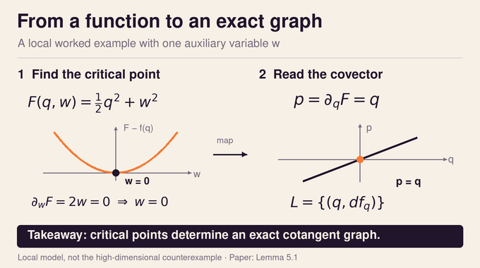
A generating family is a smooth function , with base coordinate and auxiliary variable . Its vertical critical locus determines cotangent points through
The necessary regularity is surjectivity of the full derivative of , allowing both base and auxiliary variables to vary. Individual fiber Hessians may be singular. Lemma 5.1 uses this full regularity to prove that the generated map is an immersion. On its critical locus, the pullback of equals , proving exactness.
For a simple worked example, take with scalar . The critical equation gives , and the generated image is the exact graph . More elaborate families can have multiple auxiliary solutions above one base point. Regularity controls the differential of the generated map, but distinct solutions could still produce the same cotangent point. Global injectivity needs its own argument.
The example separates three obligations. The critical equations must define a smooth locus of the correct dimension, the generated differential must be injective, and distinct critical points must have distinct images. Exactness follows locally from the generating formula, while the last obligation remains a global question.
5. Stable Tube Spaces: The Information Ordinary Topology Misses
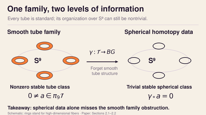
Outside a fixed auxiliary ball, the paper uses degree-two homogeneous functions , indexed by . Zero is a regular value of the angular function . Its negative domain on the unit sphere is isotopic to the negative domain of a quadratic form with negative and positive directions.
That standard domain is diffeomorphic to : a sphere core thickened by a disk. Adding positive and negative quadratic variables stabilizes these domains. Their stable smooth tube space is .
Retaining only each domain’s sphere homotopy type produces a stable spherical fibration, classified by . Here denotes stable homotopy self-equivalences of spheres. This map forgets smooth tube information. Individual domains can all be standard while their organization over the parameter sphere remains nontrivial. The proof exploits that family-level discrepancy, rather than an exotic homotopy type of a single domain.
There is a regularity subtlety here. A homogeneous function defined from smooth angular data need only be continuously differentiable at the origin. Direct sums can also lose smoothness along coordinate axes. The manuscript keeps a continuously differentiable tube model and later supplies controlled angular smoothing when smoothness away from the total origin is needed.
6. Where the Nonzero Obstruction Comes From: Waldhausen and Rognes
Waldhausen’s tube fibration relates these spaces by the homotopy fiber sequence
The first space is the stable smooth h-cobordism space of a point. Its ninth homotopy group identifies with the tenth smooth Whitehead group. Proposition 2.2 uses the exact sequence’s connecting map .
Bott periodicity gives . The stable -homomorphism is injective in both degrees. Meanwhile, , an eight-element group. Its order-two -image lies in the kernel of , so the connecting map’s image has at most four elements.
The cited Rognes computation gives the target’s two-primary part as , with 32 elements. The connecting map cannot be surjective. Exactness therefore forces
This argument establishes existence without claiming to compute every element of . It also gives injectivity of , needed next.
The counting argument can be read as a concrete obstruction test. A map whose image contains at most four elements cannot exhaust a subgroup with 32 elements. The long exact sequence then turns the failure of surjectivity into a surviving tube class. No numerical approximation enters this inference.
7. Why a Single Nondegenerate Critical Point Cannot Hide the Obstruction
Proposition 3.1 considers smooth families on , indexed by , with . Assume uniform homogeneity at infinity, exactly one smoothly varying nondegenerate critical point per fiber, and trivial stable spherical class. The proposition concludes that the stable tube class vanishes.
First, compactly supported changes move the critical point to zero, subtract its value and install its quadratic model locally. Gradient estimates ensure these adjustments introduce no new critical points or changes at infinity.
Morse theory identifies the Morse index with the number of negative directions at infinity. More precisely, the negative eigensphere bundle at the critical point is fiber homotopy equivalent to the negative-domain family at infinity. Its spherical class therefore vanishes. Injectivity of the stable -map over makes the corresponding stable negative-eigenspace class vanish too.
The dimension assumptions lift that conclusion to the required finite Grassmannian. A controlled radial interpolation then makes the local quadratic form constant across parameters. This prepares the global cobordism argument.
The lower bound on the index is used to work within a reliable stability range, rather than to optimize the dimension. Without that range, stable triviality of a vector bundle would not automatically provide the finite-dimensional deformation of quadratic forms required by the next stage.
8. From Morse Theory to a Trivial Family of h-Cobordisms
Between the fixed inner quadratic region and the outer homogeneous region, the regular zero level forms a family of cobordisms. Suitable flows identify each member with the region between an embedded inner negative tube and the outer negative tube.
Both boundary inclusions are homotopy equivalences, making these h-cobordisms. Individual product structures are insufficient: the products must vary consistently over the entire parameter sphere.
Section 4 thickens the family by one interval and extends it into a fixed sphere cylinder. A transverse flow proves that its complement is a product over the possibly varying outgoing-boundary bundle. Stability and connectivity estimates detect the original ninth homotopy class, so the original cobordism family itself admits an incoming-relative product trivialization.
Shrinking the product collars leaves small neighborhoods of the sphere cores. Additional positive quadratic variables provide enough codimension to straighten the cores through embeddings, uniformly in the parameters. The domains become a fixed tube, forcing stable nullity. This finishes Proposition 3.1 without confusing fiberwise triviality with triviality of a family.
The distinction between a product fiber and a product family is essential. Choosing a product separately for each parameter may produce incompatible choices around the parameter space. The extension and stability argument removes this compatibility obstruction before any shrinking of collars or straightening of cores is performed.
9. Constructing the Counterexample Over a Product of Spheres
Choose a representative of in a sufficiently stabilized stage with . Arrange its functions to be a fixed quadratic form near both critical points of a height function on . Set .
Over , smooth the functions near the auxiliary origin and add a cutoff version of the linear coupling . The constants are chosen in order: first , then , then the cutoff radius. Gradient bounds exclude critical points from the inner smoothing region and outer cutoff region. Every critical point satisfies
Homogeneity parameterizes the complete critical locus by : take and . The inverse recovers . Tangential variations of , together with radial variation of , prove full regularity. Thus the critical locus is diffeomorphic to the base and generates an exact immersion.
This parameterization identifies the abstract critical locus with the product of spheres. It does not assert that its projection to the original base coordinates is a diffeomorphism. Multiple auxiliary branches over one base point are allowed, provided their generated momenta separate them. That is exactly what the following argument checks.
10. Why the Constructed Lagrangian Has No Self-Intersections
Proposition 5.2 separates possible collisions using two momentum components. Equal cotangent images first require equal base coordinates . Equality of sphere momenta then forces for a scalar , since those momenta detect every component perpendicular to .
Next compare momenta in the directions. The difference contains the term . The remaining contribution is bounded by , using the uniform gradient bound and a mixed-derivative bound with constant .
Outside the fixed-quadratic neighborhoods, . Choosing makes equality of these base momenta impossible unless . Inside those neighborhoods, the fixed nondegenerate quadratic gradient already has a unique solution for each .
The immersion is therefore injective everywhere. Its critical locus is compact without boundary, so the injective immersion is an embedding with closed image. Exactness follows from the generating-family primitive. The tube class at infinity remains .
11. Transporting Generating Families Through Hamiltonian Isotopy
A hypothetical Hamiltonian isotopy must preserve the obstruction through a justified transport procedure. Section 6 extends the reverse motion to a Euclidean neighborhood of the product of spheres and divides it into finitely many small steps.
For each step, mixed generating coordinates introduce auxiliary displacement and momentum variables , contributing the nondegenerate split quadratic form . Spatial buffers and logarithmic cutoffs keep the construction inside its base domain. Direct estimates prove that the new critical locus corresponds diffeomorphically to the old one, with no unintended solutions.
The resulting functions need smoothing to recover exact homogeneity at infinity. A uniform lower gradient bound lets that smoothing occur away from all critical points, through regular homogeneous data. Split stabilization and this controlled homotopy preserve the stable tube class on every fixed compact parameter slice. Preservation is established step by step, rather than assumed for arbitrary changes of generating family.
The cutoff estimates serve two purposes simultaneously: they prevent extra critical points and retain the chosen behavior at infinity. Preserving only the generated image near its compact critical locus would not suffice, because the contradiction depends on the stable class carried by the entire parameterized family at infinity.
12. The Final Contradiction: Why Hamiltonian Isotopy Cannot Exist
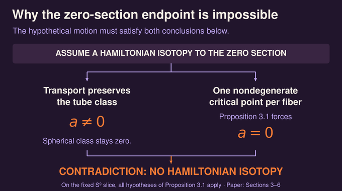
At the zero section, the transported critical-locus projection would be a diffeomorphism. Each base fiber would consequently have exactly one critical point. Its Hessian must be invertible: a nonzero vertical Hessian kernel would give a tangent vector killed by that projection.
Restrict to one fixed slice. The family retains the nonzero stable tube class , while its spherical class remains zero. Proposition 3.1 says a one-critical-point family with those properties has zero tube class. This contradiction rules out the isotopy.
The resulting obstruction concerns how a smooth manifold sits inside its cotangent bundle. Homotopy equivalence, simple homotopy equivalence and even an abstract diffeomorphism leave room for this additional structure. The proof succeeds by recording that structure in a stable family, realizing it without double points, and proving that a Hamiltonian deformation could not erase it. Each of those steps is necessary: a nonzero homotopy class alone would not produce a counterexample, and an exact immersion alone would not meet the conjecture’s embedding requirement.
The nearby Lagrangian conjecture proof disproves the unrestricted formulation through a high-dimensional construction. It leaves the cited positive low-dimensional results intact and supplies no minimum dimension. Compare the role of precise scope in our generalized Lax counterexample and Shub entropy counterexample explainers. Follow Binary Verse AI for research explanations that connect the original problem, the missing invariant and the argument that finally distinguishes them.
Is the nearby Lagrangian conjecture true or false?
The OpenAI paper gives a counterexample to the unrestricted conjecture. It constructs a closed exact smoothly embedded Lagrangian in a cotangent bundle that is not Hamiltonian isotopic to the zero section. This high-dimensional theorem does not negate every restricted case.
What does “nearby” mean in the nearby Lagrangian conjecture?
It refers to Lagrangians inside a cotangent bundle relative to its zero section, rather than a requirement of small geometric distance. The conjecture asks whether every closed exact embedded Lagrangian can be transformed into the zero section by Hamiltonian isotopy.
How can two diffeomorphic Lagrangians fail to be Hamiltonian isotopic?
A diffeomorphism describes the abstract smooth structure of a manifold. Hamiltonian isotopy additionally requires a particular type of deformation inside the surrounding symplectic manifold. The counterexample separates these conditions: its Lagrangian is diffeomorphic to the base, but its embedding is not Hamiltonian isotopic to the zero section.
Why does the OpenAI proof use S⁹ and a sufficiently large even dimension?
The S⁹ factor indexes a nontrivial stable tube class obtained from homotopy-theoretic calculations. The additional sphere factor enables the exact embedded construction. The manuscript proves existence for some sufficiently large even N, without identifying a smallest possible value.
What role does Waldhausen’s tube fibration play in the proof?
It relates the stable smooth tube space to stable spherical fibrations and stable h-cobordisms. The paper uses this relationship to obtain a nonzero smooth tube class whose associated stable spherical-fibration class vanishes. This discrepancy supplies the obstruction to Hamiltonian isotopy.
Does the counterexample overturn every known positive result about exact Lagrangians?
No. It disproves the unrestricted assertion using a high-dimensional example. Positive results for particular base manifolds, including the low-dimensional cases cited in the paper, and theorems about homotopy properties of cotangent projections remain separate results.