
A neuron can be simple while the landscape of its possible weights is anything but. Give it thousands of random inputs, constrain its weight vector to a sphere, and even calculating its equilibrium statistical weight becomes a research problem.
OpenAI’s spherical perceptron proof identifies an exact variational formula for that model’s limiting pressure, often discussed as free energy. The September 24, 2026 manuscript covers every fixed positive pattern density and inverse temperature, with any bounded continuous single-pattern potential. It proves convergence in expectation and probability. The achievement is a rigorous thermodynamic characterization, rather than a demonstrated training speedup or a storage-capacity calculation.
Table of Contents
1. What Did OpenAI Prove About the Spherical Perceptron?
Theorem 1 in The Free Energy of the Spherical Random Perceptron turns a high-dimensional random integral into an optimization over monotone functions. Neither convexity, concavity nor symmetry of the potential is required. These assumptions matter because they determine which irregular reward landscapes the theorem actually covers.
1.1. Spherical Perceptron: Key Facts And Theorem Scope
| Research Detail | Verified Scope |
|---|---|
| Weights | Real vectors with Euclidean norm . |
| Disorder | Independent standard Gaussian patterns. |
| Parameters | Fixed and . |
| Potential | Any bounded continuous real-valued function. |
| Conclusion | Exact limiting pressure, in expectation and probability. |
| Excluded Inference | No automatic hard-constraint, zero-temperature or jamming result. |
Expectation averages over the random patterns. Convergence in probability additionally says that atypical instances become unlikely. Neither statement alone promises a useful finite-size error bar for an experiment. The distinction between a theorem and a capability demonstration also guides our coverage of AI mathematical proofs.
The manuscript belongs to the collection introduced in OpenAI’s mathematics release announcement. Its theorem fixes density and temperature before taking the large-system limit. It does not establish one uniform error estimate over all parameter choices, or justify taking temperature to zero while dimension grows.
2. The Spherical Perceptron Model: Random Patterns, Weights And Free Energy
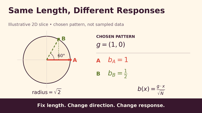
Let count weight coordinates and count patterns. The weight vector belongs to . Each independent Gaussian vector produces a scalar response:
For any fixed allowed weight, that response has a standard normal distribution. The normalization prevents its variance from growing with dimension. A prescribed potential rewards or penalizes the response, and the Hamiltonian adds those contributions:
For example, is allowed. Its reward saturates, remains bounded and distinguishes positive from negative responses. A quadratic penalty without truncation is unbounded and falls outside this theorem.
With the uniform probability measure on the sphere, define:
The partition function totals weighted spherical volume. Pressure balances reward against how much volume realizes it. The physical free energy per coordinate is . Larger inverse temperature strengthens reward preferences.
3. The Original Free Energy Problem And Earlier Replica Predictions
Gardner’s original storage-volume problem studied which neural-network weights satisfy random constraints. Later statistical-mechanics calculations described more complicated equilibrium landscapes through replica symmetry breaking, allowing similarities between independently sampled configurations to occupy multiple levels.
Györgyi and Reimann’s continuous replica-symmetry-breaking work supplied the relevant prediction in 2000. The new manuscript identifies its terminal evolution and spherical entropy with the two terms of its own pressure formula, after reconciling sign conventions.
Earlier rigorous work by Shcherbina and Tirozzi addressed restricted hard-constraint and regularized settings. Montanari and Zhou later derived related finite-temperature expressions while proving algorithmic results for exceptional Gaussian projections. Those achievements concern different observables or proof scopes. The present contribution establishes the microscopic quenched pressure for arbitrary bounded continuous rewards.
The word quenched specifies the order of averaging: take the logarithm of the partition function for each disorder realization, then average. Taking the logarithm after averaging instead gives an annealed quantity, generally a different answer. Random constraint problems, including the random 3-SAT threshold, make that distinction consequential because favorable rare instances can distort an average partition function.
4. Why Earlier Methods Could Not Establish The General Formula
Gaussian inputs do not guarantee a Gaussian Hamiltonian. Applying a nonlinear potential to each response generally destroys that property. Matching a covariance function therefore does not justify importing a Gaussian mixed-spin pressure theorem.
A second difficulty is the absent comparison sign. Standard interpolation arguments often exploit convexity or positivity to control a remainder. An arbitrary bounded continuous potential supplies neither automatically. The proof needs another way to order candidate descriptions.
This separates the problem from the Gaussian Sherrington–Kirkpatrick setting discussed in our QAOA and Parisi-limit explainer. It also explains why the related Mézard–Parisi formula for diluted spin glasses offers useful cavity intuition without directly proving this theorem. Here, adding patterns and adding weight coordinates require different arguments.
5. Understanding OpenAI’s Exact Variational Formula
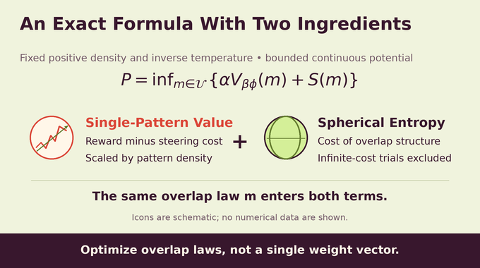
Set . An admissible order parameter is a measurable nondecreasing function from to . It represents a cumulative overlap law. Define its integrated tail and spherical entropy cost by:
The entropy integral is nonnegative and may be infinite. Trials with infinite entropy cannot improve the infimum. No requirement forces to equal one near the endpoint.
The remaining term is a single-pattern stochastic-control value. With standard Brownian motion, it is:
Controls may use information available up to the current Brownian time and must have finite expected displayed cost. They trade a better terminal reward against a quadratic steering penalty. Brownian time is an auxiliary calculation parameter, not training time.
The set contains the admissible functions just described. This spherical perceptron variational formula optimizes an entire overlap distribution, not a single preferred weight. It does not assert that every potential needs a nontrivial hierarchy.
A useful trial is throughout. Then , its entropy cost vanishes, and . This reproduces the elementary annealed upper bound. More structured overlap laws can improve it. By contrast, choosing gives an infinite entropy cost, despite a perfectly finite single-pattern reward. Optimizing the reward term alone would therefore solve the wrong problem. The two terms must be evaluated together.
6. How Overlaps, Ultrametricity And Ruelle Cascades Organize The Proof
Draw two independent weights from the same Gibbs distribution, conditional on the patterns. These are replicas. Their overlap measures alignment, with self-overlap one. Fresh Gaussian pattern responses have this overlap as their conditional covariance.
Small Gaussian perturbations enforce the Ghirlanda–Guerra identities in limiting overlap arrays. These identities describe how another replica joins the existing similarity structure. Panchenko’s results then yield nonnegative, ultrametric limiting overlaps. Finite-system overlaps need not already have those properties.
Ultrametricity organizes samples into nested clusters. Ruelle probability cascades provide random hierarchical weights for evaluating that structure. Shared ancestral Gaussian marks encode correlations, while each replica visit retains independent residual noise. Two visits choosing the same leaf still require fresh residual draws. Dropping them would change field variances and invalidate the calculation.
A one-point overlap law is the replica-symmetric special case. Allowing a distribution of overlaps permits more detailed organization when equilibrium requires it. The variational framework accommodates both possibilities. It does not assume a complicated phase diagram for every reward, nor does an illustrative cascade determine the optimizing law for a particular potential.
7. The Single-Pattern Value: Brownian Control And Tail Ordering
Adding one independent pattern changes log partition by a log Gibbs average of its exponential reward. Cascade recursion computes that increment by integrating Gaussian levels backward from the terminal potential.
For smooth terminal data, the recursion satisfies a Parisi-type backward partial differential equation. Completing the square in Itô’s formula identifies its value with the Brownian control problem above. This supplies an ordinary probabilistic calculation without continuing an integer replica count to zero.
The crucial comparison uses overlap quantiles and , not cumulative functions. For denoting the same value in quantile coordinates, the order is:
The direction matters: larger upper-tail integrals produce a smaller single-pattern value. The proof derives this from nondecreasing squared martingale means and summation by parts. That order property supplies the comparison sign missing from arbitrary potentials.
8. Deriving The Spherical Entropy And Linear-Field Formula
The entropy term must match an actual integral over a sphere. The manuscript evaluates a spherical system exposed to hierarchical Gaussian linear fields, using a canonical Gaussian calculation and radial comparison to recover the fixed-radius integral.
Its limiting field value is a dual minimum involving spherical entropy minus a field-overlap pairing. Stationary-field equations identify the field associated with a trial quantile. This connects the geometric cost of occupying the sphere with the covariance needed by the cavity argument.
The estimate is uniform for monotone quantiles bounded away from one, rather than merely valid separately for each finite hierarchy. That uniformity lets the proof enlarge its cavity after taking the bulk limit. Pointwise convergence alone would not justify that step.
More explicitly, let be an overlap quantile and let denote the same integrated cumulative function in this parametrization. The stationary relation is , where . The field covariance levels are . Keeping that factor of two is essential: losing it would make the entropy derivative and the cavity field disagree even if both separate calculations looked plausible.
8.1. Normalization Checks For Perceptron Free Energy
| Check | Required Result |
|---|---|
| Zero potential | , because the sphere measure has total mass one. |
| Constant potential | gives . |
| General reward | Lower: . Upper: . Here is standard normal. |
The last bounds follow from Jensen’s inequality. They are useful implementation checks before attempting numerical optimization, not performance benchmarks.
9. The Upper Bound: Poissonization, Contact Comparison And Synchronization
For the upper bound, the proof temporarily makes the number of patterns Poisson distributed. Differentiating expected pressure with respect to density then becomes an exact add-one-pattern calculation. Density serves as the evolution variable.
Poissonization is a proof device, not a change to the final theorem’s pattern model. A random count makes a density derivative accessible through a single new constraint. The comparison ultimately returns to the prescribed count, whose fluctuations relative to the Poisson version have negligible pressure cost per coordinate.
An enriched model adds a cascade Gaussian field. At a contact minimum of a comparison function for negative pressure, curvature and concentration enforce joint overlap identities. Synchronization orders the spin overlaps and cascade-label overlaps through a monotone coupling.
These orders imply the tail-integral inequality from Section 7. Its single-pattern comparison conflicts with the derivative inequality that a failed upper bound would require. The contradiction establishes the desired pressure bound without a convexity assumption on the reward.
Then approximation and concentration
10. The Lower Bound: Two-Pattern Removal And Spherical Geometry
The other direction asks what happens when new weight coordinates enter the system. Their effective field depends on derivatives of the pattern potential. Its covariance must be identified, rather than guessed from the original Hamiltonian.
The proof removes two patterns and restores them as independent Gaussian marks. First and second moments show that off-diagonal derivative-field covariance becomes a deterministic, nonnegative, nondecreasing function of spin overlap. The second-moment identity upgrades a conditional-mean calculation to actual identification.
Tangential integration on the sphere then connects that covariance with the derivative of spherical entropy. For smooth compactly supported potentials, the same identities keep limiting overlaps uniformly below one. This is precisely the separation needed for the uniform field calculation. Geometric integration and probabilistic removal therefore deliver matching pieces of one lower bound.
The manuscript makes the separation quantitative in its smooth proof: if , the limiting overlap support lies at or below . This bound concerns the perturbed subsequential limits used in that argument. It is not a universal empirical estimate for trained networks. Its role is to keep the covariance evaluation inside the region where the spherical-field approximation is uniformly controlled.
11. Completing The Proof: Cavity Increments, Telescoping And Convergence
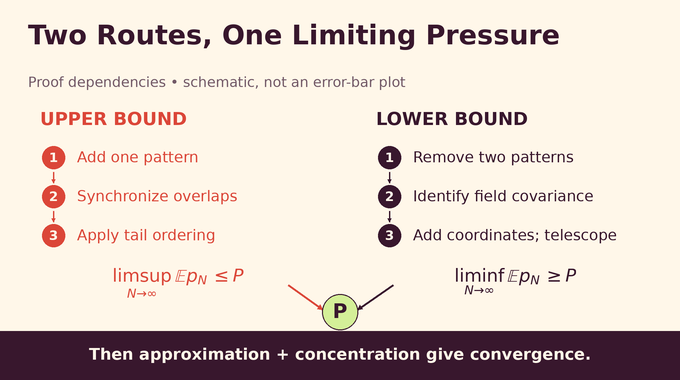
Add a fixed block of coordinates, take the bulk dimension to infinity, and evaluate the resulting cavity increment. Averaging perturbation parameters makes increments telescope. Only afterward does tend to infinity. The resulting lower bound matches the upper variational value.
Smooth compactly supported potentials were a working assumption for the derivative calculations. The final section removes it through approximation on compact sets, Gaussian integrability and uniform control-value estimates. Replacing one pattern changes log partition by a bounded amount, yielding pressure variance of order and hence convergence in probability.
Approximation here requires care. A bounded continuous function need not be uniformly approximable on the entire real line by compactly supported functions. The proof instead combines approximation on compact intervals with Gaussian tail control for pressure and second-moment bounds for controlled terminal positions. This is what extends the result beyond smooth rewards without quietly strengthening its assumptions.
The family 222 formalization documentation reports the spherical variational theorem and both convergence statements as formalized, alongside a supporting spherical-field result. Its separate Ising entry covers only finiteness. The spherical comparator configuration points to a solution module whose main theorem has a proof body. We have not independently compiled or reproduced the complete Lean verification. As in our guide to Lean proof verification, stated scope and reproduced checking remain distinct evidence.
A numerical study can now test whether its discretized variational values respect the zero-potential and constant-potential cases, the elementary bounds, and refinement of the overlap grid. Agreement is a useful diagnostic. It would still need separate numerical error analysis before being reported as an accurate evaluation for a nontrivial reward.
For researchers, the formula supplies a rigorous equilibrium target. For developers, numerical discretizations still need convergence controls. It establishes neither an efficient sampler, as studied in log-concave sampling, nor mixing guarantees like those in the switch-chain analysis. Hard constraints and jamming also need separate arguments.
The spherical perceptron now has a rigorous pressure characterization across the stated reward class. Its practical value begins with knowing exactly which quantity has been determined. Follow Binary Verse AI for research explainers that connect each theorem’s mechanism, assumptions and limits.
What is a spherical perceptron?
A spherical perceptron is a mathematical model whose weight vector has fixed Euclidean norm. In this paper the norm is , and the weights interact with independent Gaussian patterns through a prescribed potential.
What does OpenAI’s spherical perceptron proof establish?
The manuscript proves an exact variational formula for limiting pressure at every fixed positive pattern density and inverse temperature, for every bounded continuous single-pattern potential. Pressure converges in expectation and probability.
Was the spherical perceptron free energy formula known before OpenAI’s proof?
A continuous replica-symmetry-breaking formula had previously been predicted, notably by Györgyi and Reimann. The new theorem rigorously identifies the microscopic limiting pressure in the bounded continuous setting it specifies.
Why is calculating the spherical perceptron’s free energy difficult?
Although the patterns are Gaussian, applying a nonlinear potential generally produces a Hamiltonian that is not a Gaussian process. Standard Gaussian spin-glass pressure formulas therefore cannot be applied directly.
What role does replica symmetry breaking play in the proof?
Hierarchical probability cascades represent limiting overlap structures. The Ghirlanda–Guerra identities and ultrametricity help characterize Gibbs overlaps and evaluate the variational quantities. The theorem does not say that every allowed potential requires a nontrivial hierarchy.
How does OpenAI prove the upper and lower free energy bounds?
For positive log-partition pressure, the upper bound uses a density-based contact comparison and an order property of the single-pattern value. The lower bound uses two-pattern removal, spherical integration identities and telescoping cavity increments. Physical free energy has the opposite sign after division by inverse temperature.
Does the proof solve the perceptron storage-capacity or jamming problem?
Not directly. This theorem concerns finite-temperature pressure for bounded continuous potentials. Hard constraints, zero-temperature limits and microscopic jamming require additional results and do not follow from this theorem alone.