

Two neighbors can share no prime factors and still conceal a statistical dependence. The Erdős–Pomerance conjecture asks whether the relative sizes of their largest prime factors eventually behave independently. OpenAI’s September 24, 2026 preprint, The joint Dickman law for consecutive integers, proves the predicted product law in ordinary natural density. Its striking consequence: each neighbor has the larger prime factor half the time, asymptotically.
The advance removes exceptional averaging scales and additional conjectural assumptions. Understanding it requires following how prime-factor labels become a weighted graph, and why a persistent correlation would contradict known short-interval cancellation.
Table of Contents
1. What Is the Erdős–Pomerance Conjecture?
Write for the largest prime divisor of an integer , and set by convention. For example, gives , while gives . The ordering reverses immediately afterward: is smaller than .
Consecutive integers are coprime, meaning their greatest common divisor is one. Nevertheless, excluding shared divisors does not prove independence between the sizes of their largest divisors. Disjoint ingredients can still produce dependent measurements.
The conjecture concerns logarithmically normalized sizes, not independent complete factorizations. Normalization asks what power of the integer is needed to reach its largest prime factor. This makes comparisons across very different numerical scales meaningful. Our two-point Chowla explainer examines another statistic of neighboring factorizations, their parity. Here the question concerns the largest prime factor of n and n+1.
1.1. Erdős–Pomerance Conjecture: Key Facts
| Problem | The Erdős–Pomerance joint Dickman conjecture concerns the largest prime factors of consecutive integers. |
|---|---|
| Research Source | OpenAI’s preprint dated September 24, 2026, especially Theorem 1.1 and Corollary 1.2. |
| Main Conclusion | The two normalized largest-prime-factor statistics have independent limiting distributions, each described by the Dickman function. |
| Counting Convention | Ordinary natural density, using equal weights and limits through all real counting endpoints. |
| Ordering Consequence | Each strict ordering of the two largest prime factors has natural density . |
| Assumptions | Unconditional, with each smoothness exponent fixed strictly between zero and one. |
| Formalization Scope | OpenAI’s Lean documentation identifies the joint theorem and both strict-ordering conclusions as covered targets. |
| Quantitative Limit | Theorem 1.1 asserts convergence without specifying an error rate or uniformity for growing parameters. |
2. The Dickman–de Bruijn Function and the Distribution of Largest Prime Factors
An integer is -smooth when every prime factor is at most . Thus 60 is 5-smooth, even though its numerical size greatly exceeds five. Smoothness measures the sizes of the ingredients, not the finished product.
The Dickman–de Bruijn function supplies the limiting frequency of such integers. It is continuous and determined by:
This delay differential equation uses the function’s value one unit earlier to determine its slope. On the first interval after one, it gives for . Throughout this article, means the natural logarithm.
For fixed , the classical single-integer law is:
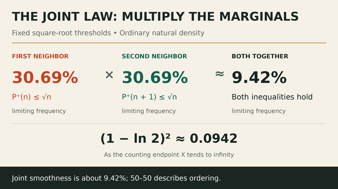
Here denotes the number of qualifying integers. With , the limiting proportion is , approximately 30.69 percent. This established marginal distribution is the starting point. Knowing it separately for both neighbors still leaves their joint behavior unanswered.
3. What OpenAI’s Joint Dickman Law Actually Proves
Theorem 1.1 fixes two real numbers . Defining the normalized joint count makes its statement readable:
Both thresholds deliberately use , including the threshold for its successor. Equivalently, the measured coordinates are and . The second can slightly exceed one at finite inputs, but that overshoot vanishes asymptotically.
Ordinary natural density gives each integer equal weight and divides the count by . The endpoint tends to infinity through all real values. At , the product predicts approximately 9.42 percent for the joint event, not 50 percent. The half-and-half statement concerns ordering instead.
The paper appeared in OpenAI’s mathematics release. Its Lean scope documentation lists the joint law and both ordering densities. As our Fermat formalization analysis explains, formalization and discovery answer different questions. Documented scope also needs distinguishing from an independent rebuild or peer review.
4. Why Earlier Proofs Could Not Establish the Full Conjecture
Earlier progress approached the target from several directions. Positive lower density established that neither ordering becomes negligible. It did not establish convergence to a particular frequency, a distinction also central to our large prime gaps analysis.
Teräväinen’s logarithmic-density theorem obtained the product law by weighting an integer by its reciprocal and normalizing by . Such an average can converge while ordinary averages retain problematic scales. Tao and Teräväinen obtained ordinary-average conclusions outside exceptional scales, with later work supplying quantitative estimates and parameter uniformity.
4.1. Previous Results and the Missing Ordinary Limit
| Positive Lower Density | Erdős and Pomerance proved both orderings occur with positive lower density. Later bounds improved their guaranteed minimum frequency. |
|---|---|
| Logarithmic Density | Teräväinen obtained the predicted product and half-density ordering after reciprocal weighting. This does not establish the ordinary limit. |
| Exceptional-Scale Results | Tao and Teräväinen obtained ordinary-average conclusions outside a set of scales of logarithmic density zero. Later work added quantitative control. |
| Conditional Ordinary Law | Wang obtained the joint law assuming an Elliott–Halberstam conjecture for friable integers, leaving an additional unproved hypothesis. |
| OpenAI’s Theorem 1.1 | The product limit holds unconditionally, with ordinary counting and no exceptional scales, for every pair of fixed interior exponents. |
Wang’s conditional approach instead assumed an Elliott–Halberstam conjecture for friable integers. “Friable” means smooth. The new proof requires no such hypothesis. As in our Artin primitive-root discussion, removing assumptions and strengthening a counting conclusion are separate achievements.
The precise missing step was unconditional convergence of the ordinary joint average at every scale. The manuscript supplies that qualitative conclusion without importing the earlier quantitative error bounds.
5. Step 1: Encoding Large Prime Factors to Reduce the Problem to Correlation
Fix an integer and split large primes into logarithmic bins , with . Let count prime factors in that bin, including multiplicity. Unit complex phases define a multiplicative label:
A second, independently chosen phase vector defines . These are deterministic arithmetic functions. Independent choice of test phases does not assume the independence being proved.
For integers bounded by a fixed multiple of , the count vectors occupy a fixed finite set. Finite Fourier inversion therefore reconstructs every bin event from these phase tests. Centering the first label gives , where is its limiting mean. Proposition 2.2 targets:
The centered label is not multiplicative. What survives is crucial: for each fixed positive integer , eventually and . Every prime dividing that fixed multiplier eventually lies below the bins. This invariance later permits a substantial change of variables.
6. Step 2: Obtaining Cancellation Through Short-Interval Averages
The proof needs cancellation after attaching weights that will emerge from its graph construction. For an auxiliary parameter , choose a finite auxiliary-prime set whose minimum tends to infinity. For fixed , define:
Each factor averages two choices: discard the prime or retain it. If is the product of independently retained primes, each kept with probability one-half, this weight is the conditional expectation of . It is a bridge between random splitting and multiplicative arithmetic.
Lemma 2.3 gives mean-square cancellation for short averages of , including fixed residue restrictions. The base points have size comparable to , where grows. Shift-interval lengths also grow with , while remaining short compared with in the inner limit. Mean-square control averages the squared magnitude over base points. It permits exceptional intervals, provided their combined contribution vanishes. The argument therefore needs averaged local cancellation, rather than cancellation inside every individual short interval.
To access existing theorems, the proof interpolates the finite bin data using real, nonnegative multiplicative functions. Matomäki and Radziwiłł’s short-interval comparison handles principal character components. The corrected complex theorem of Matomäki, Radziwiłł and Tao handles nonprincipal twists. Centering cancels the corresponding long means.
7. Step 3: Divisor Amplification and the Emergence of Positive Energy
Assume the mixed correlation stays bounded away from zero along some sequence. Passing to a subsequence produces a bounded profile recording scaled position and compatible residue information. The latter lives on the profinite integers, a space that packages residues modulo every positive integer.
The amplifier is a nonnegative weighted count of representations and . Its coefficient windows are and . For fixed , only finitely many coefficients occur.
The weight has a positive mean and bounded second moment. Because its primes escape every fixed residue modulus, it preserves a nonzero contribution from the limiting profile. Simply inserting an arbitrary divisor weight would not justify that preservation.
Expand the weighted average and replace by . Cauchy–Schwarz removes this unit-modulus factor and produces a nonnegative quadratic energy in the centered label. Its normalized lower bound stays positive. Equal-coefficient terms contribute negligibly, leaving distinct coefficients to carry the surviving energy.
“Energy” here is a squared arithmetic sum. It is a proof device, not a physical quantity or a training objective.
8. Step 4: Transforming Divisor Relations into Additive Shifts
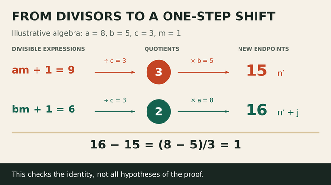
An off-diagonal pair satisfies and . Since is invertible modulo , subtracting gives for a nonzero integer . The coefficient windows ensure .
Set and . The decisive identity is:
Indeed, . Multiplication by the fixed coefficients preserves the centered labels once is sufficiently large. Thus the quadratic label product becomes a correlation between and , with the conjugation inherited from the squared sum.
The multiplicative representation problem has become a graph of additive shifts. Vertices are transformed integer endpoints, of size comparable to . Edges retain weights describing divisor choices and residue restrictions. Discarding those weights would discard the difficult part of the argument.
This is why short-interval cancellation was prepared at the larger endpoint scale. The change of variables determines precisely which averages the final contradiction must control.
9. Step 5: Independent-Site Kernels and Second-Moment Estimates
Group nearby endpoints into blocks with positions, where is a fixed sufficiently large constant. At each model position, include an auxiliary prime with probability , independently across primes and sites. The inclusion probability matches the density of multiples of .
This independence belongs to an auxiliary comparison model. Actual integer divisibility patterns remain constrained. A prime cannot divide two distinct integers whose difference is smaller than that prime. Independent model sites can share a prime, so their usefulness depends on bounding the discrepancy, rather than asserting exact equality of the models. The paper couples the arithmetic data to the model with controlled errors, then averages the extra residue weights attached to individual representations.
The resulting endpoint kernel assigns a weight to two site-prime sets and their positions. A kernel is simply a rule for weighting pairs, a viewpoint also used in our Sidorenko graph analysis.
The comparison requires more than agreement of average weights. A small number of unusually large rows could dominate later optimizations. Section 6 controls representation multiplicities, integrated squared row weights, and the second moment of total mass. It uses conditionally independent fair splits of the same prime sets, retaining shared information before averaging the separate choices.
These estimates make subsequent sampling legitimate. Replacing arithmetic by independent randomness without them would merely restate the original wish.
10. Step 6: Endpoint Features, Cut Norms, and the Final Contradiction
For a site-prime set , fairly split its primes into a product . The endpoint feature is the conditional probability that lies in a coarse interval , divided by that interval’s length. Channel estimates suppress residue dependence and approximate logarithmic outputs uniformly by these coarse features.
The kernel is then approximated by a finite sum of products of endpoint features. Its coefficients separate an arithmetic lag factor from smooth dependence on lag and block position. The required number of features is fixed before the limiting process.
An integral comparison initially controls tests depending separately on each endpoint. Actual optimizing signs may depend on the entire sampled matrix. The cut norm measures the largest normalized bilinear pairing with two vectors bounded by one. Choosing those vectors after seeing the matrix tests whether any grouping of endpoints can preserve a large hidden interaction. Cut-norm sampling, supported by the second-moment estimates, closes that gap by approximating an optimizing cut with a small sample of columns.
Finally, polynomial approximation expresses the features through finite combinations of . Periodic approximation handles the arithmetic lag factor. Subdividing blocks reduces the energy to products of the weighted short averages from Step 2, which vanish.
That contradicts the positive energy from Step 3. Throughout, tends to infinity before . As in our QAOA limit-order explainer, exchanging limits would require a separate justification.
11. Why OpenAI’s Proof Gives the 50–50 Largest-Prime-Factor Law
Finite Fourier inversion now recovers joint bin events. Refining rational thresholds and using continuity yields the joint Dickman law for consecutive integers, first at fixed counting-scale thresholds and then at the moving thresholds of Theorem 1.1.
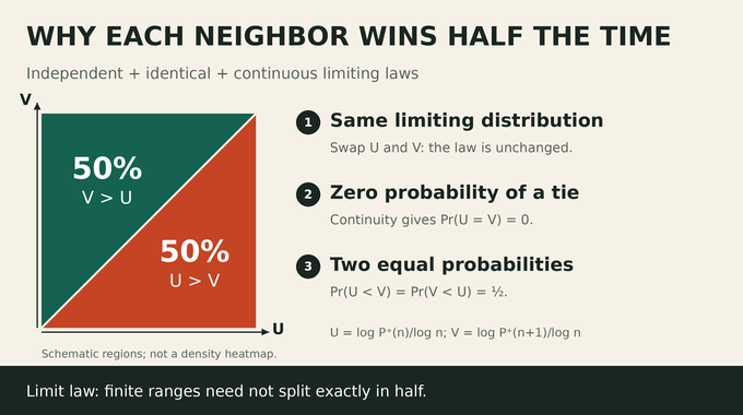
The limiting normalized coordinates are independent and identically distributed. Their common distribution is continuous, so equality has probability zero. Symmetry of this limiting pair gives equal probability to either strict ordering:
This proves the Erdős–Turán largest prime factor conjecture as Corollary 1.2. Symmetry is a property of the limiting distribution, not an assumed symmetry of finite consecutive pairs. Individual pairs remain entirely deterministic.
For researchers, the reusable insight is the passage from divisor amplification to endpoint features and short averages. Developers can explore frequencies with a sieve, but finite experiments cannot certify the limit or supply a convergence rate absent from the theorem. The result provides no factoring speedup or cryptographic performance guarantee.
11.1. What the Independence Theorem Does and Does Not Supply
| Parameters | Choose the smoothness exponents first and keep them fixed while the counting range grows. |
|---|---|
| Statistical Independence | The conclusion concerns normalized largest-prime-factor measurements. It does not assert independence of complete prime factorizations. |
| Finite Ranges | The ordering proportion need not be exactly one-half at any chosen finite cutoff. |
| Error Estimates | The theorem supplies no quantitative convergence rate or certified cutoff for a desired numerical accuracy. |
| Practical Computation | Counting examples can illustrate the law. The proof does not demonstrate an algorithmic speedup or improved cryptographic performance. |
The Erdős–Pomerance conjecture thus becomes a precise theorem about asymptotic independence of prime factors in the specified normalized statistics, with fixed parameters and no exceptional scales. Follow Binary Verse AI’s research explainers to trace more results from their original obstacle through the argument that removes it.
What is the Erdős–Pomerance conjecture?
It predicts asymptotic independence between the normalized largest prime factors of consecutive integers. OpenAI’s proof establishes the joint Dickman product law in ordinary natural density, with each smoothness exponent fixed between zero and one.
Why does coprimality not already prove independence?
Consecutive integers share no prime divisors, but this deterministic restriction does not establish independence between the statistical distributions of their largest prime factors.
Why is the Dickman function used in the proof?
The Dickman–de Bruijn function describes the limiting proportion of integers whose prime factors do not exceed a fixed power of the counting threshold. Its values supply the two marginal distributions in the joint theorem.
What was missing from previous proofs?
Earlier results established logarithmically averaged independence, conditional ordinary-density results, or ordinary-average conclusions outside exceptional scales. The new theorem establishes the full unconditional ordinary-density limit for fixed smoothness parameters.
Does the 50–50 result apply to every consecutive pair?
No. It is an asymptotic frequency statement. As the counting range grows, each strict ordering of the two largest prime factors has natural density one-half. No chosen finite range is required to split exactly evenly.
Does OpenAI’s proof require the Elliott–Halberstam conjecture?
No. The manuscript’s principal theorem is unconditional. One earlier approach required an Elliott–Halberstam-type hypothesis for friable, or smooth, integers.
Does the proof establish independence of complete prime factorizations or provide a convergence rate?
No. It proves independence of the specified normalized largest-prime-factor statistics. It does not establish independence of complete prime factorizations, and Theorem 1.1 asserts no quantitative convergence rate.