

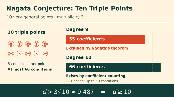
Can a degree-nine plane curve vanish three times at each of ten very general points? It has 55 coefficients facing 60 conditions, which suggests failure. Proving that those conditions really rule out every curve is the difficult part. The Nagata conjecture turns this example into a universal bound connecting degree, multiplicity, and the square root of the number of points.
OpenAI’s September 23, 2026 manuscript presents a proof for every integer , including unequal multiplicities and repeated components. Its decisive move converts geometry into interpolation on lattice points. Released through OpenAI’s mathematics announcement, the argument now also has a specialist exposition. Here is how the original paper moves from curves to a finite matrix, and precisely what its conclusion establishes.
Table of Contents
1. What Is the Nagata Conjecture for Plane Curves?
A projective plane curve is defined by one homogeneous polynomial in three variables. Its degree is the common total degree of its monomials. Multiplicity at a point means that, in local coordinates, every term of total degree below disappears. Triple points therefore require the value, both first derivatives, and all three second-order coefficients to vanish.
A degree-nine form has coefficients. Ten triple points impose at most 60 homogeneous linear conditions. Degree ten supplies 66 coefficients, so a nonzero solution to those conditions exists. This guarantees a curve, without promising smoothness or irreducibility.
The missing step is exclusion at degree nine. Excess conditions can be dependent. Nagata’s conjecture for plane curves asserts the precise inequality that supplies this exclusion for very general configurations.
| Feature | Verified Manuscript Scope |
|---|---|
| Source | OpenAI manuscript dated September 23, 2026. |
| Point configuration | Every integer , at very general distinct points. |
| Curves covered | Positive degree, including reducible curves and repeated components. |
| Multiplicities | Arbitrary nonnegative integers bounded by actual vanishing orders. |
| Main inequality | . |
| Ten triple points | Minimum degree ten. Degree nine is excluded. |
| Formalization status | Repository documentation reports the full inequality. No independent compilation was performed for this article. |
This is an interpolation problem: prescribe local behaviour and ask whether a global polynomial can meet it. Unlike interpolation in one variable, the positions and geometry of points in two dimensions can create unexpected dependencies. That is why counting coefficients provides the starting intuition rather than the proof.
2. The Exact Inequality: What the Conjecture Really Says
Theorem 1.1 of the original Nagata manuscript states that a nonzero effective curve of positive degree, with prescribed nonnegative multiplicities no larger than its actual multiplicities, satisfies:
Here counts distinct marked points and is the required multiplicity at the ith point. “Effective” allows reducible curves and components appearing repeatedly. Equal multiplicities give . For ten triple points, this requires , approximately 9.487, hence integer degree at least ten.
“Very general” means outside a countable union of proper Zariski-closed subsets of the configuration space. These exceptional subsets describe algebraic special arrangements. One exceptional union works simultaneously for every degree and multiplicity vector.
Strictness matters. A non-strict inequality would leave possible equality when is a perfect square. For nonsquare , the equal-multiplicity ratio is rational while is irrational, so equality is automatically impossible.
As of October 27, the Lean scope documentation reports formalization of this full statement. This article has not independently compiled it or established journal acceptance. That distinction also matters in our explanation of proof formalization.
3. The Previous Barrier: Why Perfect Squares Were Easier
Nagata proved the square cases for . Their geometry has a natural matching scale: a smooth degree- curve has normal bundle of degree . The number of marked points and that bundle degree align exactly.
The manuscript reproves these cases, including the strict endpoint, using coefficient vanishing and a carefully chosen degree-zero line bundle. A line bundle packages how local function descriptions glue together. Its degree controls how many zeros a nonzero section can have.
Nine points behave differently. Cubic forms have ten coefficients, so nine point conditions always leave a nonzero cubic. With simple multiplicities, degree three gives equality in the proposed bound. The strict theorem cannot start there.
For nonsquare counts, earlier methods approached the target through rational estimates. The paper records the ten-point bound , approximately 3.162162. The desired threshold is , approximately 3.162278. That small numerical gap still leaves infinitely many multiplicity levels to control. Checking finitely many examples cannot close it.
The difficulty was therefore uniformity: exclude every forbidden slope, however large the multiplicity becomes, while retaining the exact square-root boundary.
4. The First Breakthrough: Reducing the Problem to Equal Multiplicities
Fix a degree and multiplicity vector. The configurations admitting a suitable curve form a closed incidence locus: write the vanishing conditions as a matrix, then require all maximal column minors to vanish.
Outside the union of proper incidence loci, existence has a powerful consequence. If a curve with those data exists at such a tuple, its incidence locus must be the entire configuration space. Curves with the same requirements then exist at every configuration.
Next, cyclically permute the multiplicity vector. At each fixed configuration choose a curve for each cyclic shift and multiply their equations. Every multiplicity appears once at every point. The product has degree and common required multiplicity , where was the original degree.
Any violation consequently produces a universal equal-multiplicity system with . Universal means that a suitable nonzero form exists for every ordered tuple of distinct points.
This reduction also permits taking arbitrary positive powers. Both degree and multiplicity scale together, preserving their ratio. That apparently simple freedom becomes essential when the final lattice count must absorb an integer endpoint error. Unequal multiplicities are handled before the analytic machinery begins.
5. From Plane Curves to Normal-Bundle Polynomials
Choose a smooth plane curve of degree . Move the marked points toward it, with independently chosen normal displacements. Locally, a normal coordinate measures motion away from the curve, while a tangent coordinate measures motion along it.
Rescale the normal coordinate by the motion parameter. A suitable family of plane forms then has a first nonzero limiting term. The paper constructs a polynomial on the normal line bundle:
Here is the restriction of the hyperplane line bundle to , is the normal fibre coordinate, and denotes global sections. The powers ensure that the terms glue consistently across coordinate charts.
Two safeguards carry the argument. Selecting the first nonzero contribution prevents the limiting polynomial from disappearing. Tracking local derivatives proves that multiplicity at least survives at the prescribed displaced points.
The result is a necessary condition for the hypothetical universal system. Every chosen configuration on the normal bundle must admit this nonzero polynomial. Ruling out one carefully engineered normal configuration will therefore rule out the original universal plane system.
6. Why Nine Points on an Elliptic Cubic Change Everything
For nonsquare , take . A smooth plane cubic is an elliptic curve. Here it supplies complex geometry and explicit sections, rather than the arithmetic questions discussed in our elliptic curve modularity explainer.
Set the normal displacements at nine distinct points to zero and write for their sum as a divisor. Multiplicity forces coefficient , for , to vanish at each point to order at least . After those prescribed zeros are removed, all these coefficient bundles have degree .
The paper first excludes . Negative degree forbids nonzero sections. At equality, a suitable nontorsion degree-zero bundle eliminates the lower coefficients, and a tenth nonzero displacement eliminates the remaining monomial.
Now define , a degree-zero bundle, and . Writing , where vanishes at the nine points, absorbs their coefficient zeros. The transformed coefficients belong to bundles .
The first coefficient spaces now have equal positive degree and dimension. Higher coefficients occupy specified subspaces. Preserving those subspaces, rather than replacing them with larger spaces of the same degree, keeps the later exponent diagram accurate.
7. Colliding Fat Points: Turning Geometry Into Jet Conditions
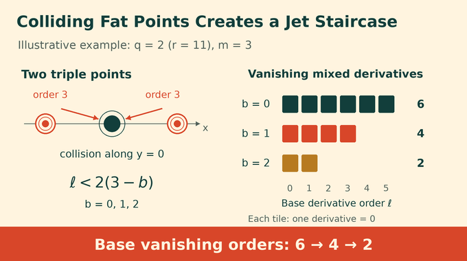
A fat point records a point together with an order of vanishing. The remaining fat points are placed along one local horizontal line on the bundle surface and brought together.
Use coordinates centred at their collision. After derivatives in the fibre direction, each original point still contributes base vanishing of order at least . Their collision therefore forces base order at least .
The resulting local ideal is . Equivalently, the required mixed derivatives are:
These derivatives are called jets: finite Taylor data at one point. They define a linear map from the transformed polynomial space to the space of required jet values. Universal existence forces this map to have a nonzero kernel on each fixed elliptic curve.
The limiting section stays nonzero because coefficient vectors are normalized in a fixed finite-dimensional space before taking a convergent subsequence. This collision occurs before the elliptic curve degenerates. Keeping those limits separate avoids assuming that kernel vectors can be chosen coherently across a changing family of curves.
8. Theta Functions and the Degeneration of the Elliptic Curve
The paper realizes each elliptic curve as the complex torus , with . Theta products give sections with prescribed zeros, and Laurent expansions give explicit bases for their line bundles.
The transformation rule of each bundle determines a recurrence between Laurent coefficients. One free coefficient per residue class produces a basis. Thus the calculation remembers the actual bundle multipliers, not merely dimensions.
Choose logarithmic coordinates near a moving base point and normalize the basis sections. As tends to zero, their local expressions approach exponentials , where integer is the fibre degree and integer is a Laurent exponent.
Convergence holds together with every fixed derivative on compact neighbourhoods. That is essential: convergence of function values alone would not justify the limit of the jet matrix.
Jenia Tevelev’s October 21 exposition reconstructs the equal-multiplicity argument and highlights theta-function asymptotics and interpolation duality as the decisive combination. His account provides a specialist route through the proof. It should not be silently equated with a separate journal review or a fresh audit of the accompanying Lean development.
9. How the Proof Becomes a Lattice-Point Interpolation Problem
Differentiate a limiting exponential at the origin. Each base derivative contributes , and each fibre derivative contributes . The limiting matrix therefore has entries:
Rows correspond to the derivative pairs allowed by the collision. Columns correspond to a finite set of exponent pairs . For each fibre degree, the allowed Laurent exponents lie in carefully specified intervals. A possible degree-zero coefficient contributes one additional endpoint pair.
| Geometric Object | Finite Interpolation Counterpart |
|---|---|
| Polynomial section | A vector of unknown coefficients. |
| Basis section | One column indexed by . |
| Collision condition | One matrix row indexed by . |
| Mixed derivative | Entry , with zeroth derivatives contributing one. |
| Forbidden curve system | A required nonzero vector in the jet map’s kernel. |
| Full column rank | Injectivity, contradicting that required kernel. |
Reading the matrix the other way, its rows evaluate allowed monomials on . Full column rank means those monomials can interpolate every assignment of values to the exponent points.
That is stronger than counting equations and unknowns. It proves independence for this structured configuration. A nonzero maximal minor in the limiting matrix stays nonzero for sufficiently small positive , so the actual jet map becomes injective. This directly conflicts with the kernel forced by the hypothetical curves.
The proof has reached an explicit finite problem, but the geometry of the exponent set must still establish its rank. An arbitrary collection of equally many lattice points would not suffice.
10. The Final Argument: Polygon Geometry, Full Rank, and Contradiction
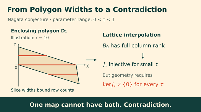
Group exponent points into horizontal rows of fixed , containing points. The interpolation lemma requires:
Treat larger rows first. Interpolate along the current row using the first coordinate, then multiply the correction by factors vanishing on previously treated heights. The two bounds keep both polynomial degrees within the allowed derivative region.
To prove those bounds, the paper encloses in a scaled, translated polygon. Its horizontal slice widths control row sizes and the number of sufficiently populated rows. Setting gives the identity , matching the slice profile to the collision parameter exactly.
For nonsquare , rationality gives . This strict gap allows contraction by a factor . Integer intervals can contribute an extra endpoint, so take a common power of the original curve until . The ratio and contraction remain fixed.
The row bounds now give full rank. The jet map must be injective for small positive parameter, yet have a nonzero kernel at every parameter. This contradiction excludes the universal system and completes the reduction back to all multiplicity vectors.
11. What the Proof Establishes for Seshadri Constants
Blow up the plane at the marked points. Let denote the pullback of a line and the exceptional curves. The theorem makes the real divisor class strictly nef: its intersection with every irreducible curve is positive. Nevertheless, its self-intersection is zero.
The multipoint Seshadri constant measures the largest equal amount that can be subtracted along all exceptional curves while keeping nonnegative intersections. Corollary 6.2 obtains:
The theorem supplies the lower bound. Elementary coefficient counting supplies curves whose ratios approach the same value, giving the upper bound. The constant is irrational whenever is nonsquare, even though every individual curve has integral degree and multiplicities.
Finally, rationally defined incidence conditions extend the conclusion to uncountable algebraically closed fields of characteristic zero. This does not require embedding every such field into the complex numbers.
The Nagata conjecture proof thus identifies an exact positivity boundary through explicit interpolation. Follow Binary Verse AI’s research proof explainers to keep the theorem, its mechanism, and its verification scope connected as you read the original mathematics.
Has Nagata’s conjecture been proved?
The September 23, 2026 OpenAI manuscript presents a proof for every integer at very general points, including unequal multiplicities. Jenia Tevelev’s October 21 exposition reconstructs the equal-multiplicity argument. The repository reports a Lean formalization of the full inequality. This article has not independently compiled that formalization or established journal acceptance. An exposition, formalization documentation, and journal peer review are distinct forms of evidence.
Why does Nagata’s conjecture require at least ten points?
Any nine points in the projective plane lie on a nonzero cubic, since cubic forms have ten coefficients and nine point conditions leave a nonzero solution. For nine simple points, , giving equality rather than the required strict inequality. The theorem therefore cannot begin at nine.
What does “very general points” mean in Nagata’s conjecture?
The points lie outside a countable union of proper Zariski-closed subsets of their configuration space. These excluded sets describe algebraically special configurations. The manuscript chooses one exceptional union that works simultaneously for every positive degree and every nonnegative integral multiplicity vector.
Can a degree-nine curve pass through ten general triple points?
No. For ten very general points with multiplicity at least three, the theorem requires , so integer degree must be at least ten. The corresponding fixed degree-nine incidence locus is proper, giving exclusion for general configurations as well. A degree-ten form has 66 coefficients facing at most 60 linear conditions, so a nonzero curve satisfying the triple-point requirements exists. It need not be irreducible or smooth.
Why couldn’t mathematicians prove Nagata’s conjecture by counting polynomial coefficients?
Counting coefficients gives an upper bound on the number of imposed linear conditions but does not prove their independence. Geometric configurations can create dependencies. The manuscript controls them through specialization to a normal bundle, collision of fat points, theta-function degeneration, and a full-column-rank interpolation matrix.
Does the proof cover unequal multiplicities and reducible curves?
Yes. Theorem 1.1 covers arbitrary nonnegative prescribed multiplicities bounded by actual multiplicities, as well as reducible and nonreduced effective curves. A cyclic-product reduction converts any hypothetical violation into a universal equal-multiplicity system, which the later argument excludes.
What does the proof establish about Seshadri constants?
For very general points of the projective plane, Corollary 6.2 gives the exact multipoint Seshadri constant of the line bundle as . This value is irrational whenever is not a perfect square. The statement also extends to uncountable algebraically closed fields of characteristic zero.