

Six jobs, three machines, and a dependency chain can still leave processors idle. The difficulty is choosing which available work to run now without delaying the finish later. Three machine scheduling turns that familiar coordination problem into a precise mathematical question: can an optimal schedule always be found in polynomial time?
OpenAI’s September 24, 2026 research paper answers yes for nonpreemptive, unit-length jobs with arbitrary acyclic dependencies on three identical parallel machines. Its deterministic algorithm decides deadline feasibility and constructs a minimum-makespan schedule. The proof bounds the information needed to describe recursive subproblems. Its enormous runtime exponent establishes theoretical solvability, without establishing practical speed.
Table of Contents
1. What Is Three Machine Scheduling, and Why Was It Open for 47 Years?
The question appears as OPEN8 in Garey and Johnson’s 1979 catalogue of computational complexity problems. Counting from that publication to 2026 gives the headline’s 47 years. Earlier formulations already existed, so 1979 is a historical reference point, not a claim about the problem’s first appearance.
Scheduling looks deceptively close to sorting: arrange the jobs so every prerequisite comes first. But a valid order alone does not determine how to pack jobs into parallel slots. Different packings can create different amounts of unavoidable waiting. The target is the earliest possible final completion, not merely a schedule that obeys the rules.
| Feature | Verified Scope |
|---|---|
| Input | An explicitly listed acyclic directed graph of nonempty, unit-length jobs. |
| Resources | Three identical parallel machines; one uninterrupted job per machine per slot. |
| Guarantee | Exact deadline feasibility and construction of a minimum-makespan schedule. |
| Runtime measure | Deterministic multitape Turing-machine steps in total binary input length. |
| Practical evidence | The paper supplies no practical running-time guarantee or competitive benchmark. |
2. The Unit-Job Scheduling Problem: Three Machines, Dependencies, and Makespan
Let be the directed acyclic graph, or DAG, with jobs. An edge from to requires to finish before starts. A schedule assigns each job a slot through . For every precedence edge and every slot from one through the deadline, the constraints are:
Slot executes during . Every job lasts exactly one time unit and cannot be interrupted. Machines are interchangeable, so the slot assignment contains the essential scheduling information. Makespan is the last completion time. Minimum makespan scheduling seeks the smallest feasible .
The model excludes release dates, communication delays, machine eligibility restrictions, and extra resources. Allowing real-valued start times would not improve this optimum: preserving a feasible schedule’s machine orders and starting each job as early as its predecessors permit yields integer start times without delaying completion.
3. Why Two Machines Were Solved but Three Remained Difficult
The two-processor case had polynomial algorithms decades ago, including Coffman and Graham’s 1972 optimal list-scheduling algorithm. Those results did not settle three processor scheduling with arbitrary dependencies. An additional machine changes the packing choices enough that the earlier structural guarantees no longer supply a general solution.
Restricted precedence structures remained useful footholds. Opposing forests, formed from disjoint in-forests and out-forests, admit a linear-time three-processor algorithm. Dolev and Warmuth obtained polynomial time when both precedence height and machine count are fixed. Arbitrary DAGs need not satisfy either restriction.
Nederlof, Swennenhuis, and Węgrzycki’s SODA 2025 exact algorithm achieved subexponential time for fixed machine count. It already decomposed schedules and memoized structured subproblems. The new polynomial result builds on that viewpoint, rather than deriving its bound by substituting three into the earlier runtime.
Approximation schemes supplied another route, permitting a chosen small multiplicative loss in makespan. Exactness matters here. As in our shortest common superstring explainer, a polynomial approximation guarantee and an exact optimum are different promises.
4. What OpenAI’s Polynomial-Time Scheduling Proof Establishes
Theorem 1.1 assumes an explicitly listed finite DAG on jobs. Given an integer deadline , a uniform deterministic algorithm decides feasibility exactly and returns a schedule whenever feasible. It also constructs an optimal schedule without a supplied deadline. Both tasks fit the bound:
Here is the total binary input length. “Uniform” means one fixed algorithm handles every valid input size. There is no separate magical solver for each graph size, and no randomized success probability.
The theorem therefore establishes a polynomial time scheduling algorithm for this model. It supplies the schedule itself, not merely its length. That witness requirement also matters in maximum cardinality matching. Finding an optimum, deciding feasibility, and counting configurations remain distinct computational tasks.
5. A Worked Three-Machine Scheduling Example
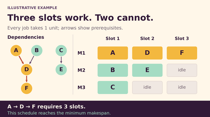
Consider six jobs named A through F. The dependency arrows are A → D → F, B → D, and C → E. These are illustrative jobs chosen here, not an experiment reported in the paper. Every job takes one time unit.
| Machine | Slot 1: [0, 1) | Slot 2: [1, 2) | Slot 3: [2, 3) |
|---|---|---|---|
| Machine 1 | A | D | F |
| Machine 2 | B | E | Idle |
| Machine 3 | C | Idle | Idle |
A, B, and C can run together immediately. D then waits for A and B, while E waits for C. F must wait until D finishes. The table respects every dependency and finishes at time three.
No two-slot schedule can work because A → D → F is a chain of three unit jobs. Thus three is both an achievable makespan and a lower bound, proving optimality. The empty positions reflect dependencies, despite sufficient aggregate machine capacity for six jobs in two slots.
This example checks the model. Larger instances need the new proof because obvious workload and longest-chain lower bounds alone do not generally identify an optimal packing.
6. The First Breakthrough: Turning Schedules Into Independent Intervals
Fix a candidate deadline . If , reject immediately: three machines cannot complete that many unit jobs. Otherwise add isolated dummy jobs, producing jobs. The dummies have no dependencies and fill otherwise vacant positions.
The padded instance is feasible exactly when the original deadline is feasible. Every slot can now be treated as a full triple of mutually incomparable jobs. Removing the dummy jobs later recovers an original schedule.
Mark selected triples as boundaries. Jobs strictly between consecutive boundaries form an open interval. Replacing that interval’s internal schedule with another feasible schedule of exactly the same jobs preserves feasibility globally: every exterior job remains before or after the entire interval.
That replacement lemma is simple. Naming the interval is harder. Its boundary triples do not uniquely identify its job set. Remembering every ancestor interval could require descriptions that keep growing, defeating a polynomial dynamic program. The proof must compress that inherited information without losing jobs or admitting outsiders.
7. Shared-Cutoff Separators: How the Proof Preserves Dependencies
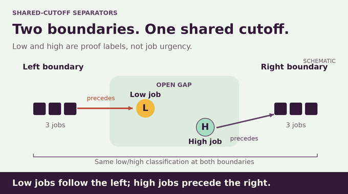
Choose a priority order extending precedence, meaning every predecessor ranks before its successors. An initial segment contains the low jobs, and the remaining jobs are high. These labels track a moving cutoff, rather than processing duration or business importance.
A selected slot separates the cutoff when every earlier high job precedes a job in that slot, and every later low job succeeds a job there. These are precedence relationships. Simply occurring earlier in time does not imply being a prerequisite.
The proof considers a normalized schedule: among feasible arrangements, choose the lexicographically earliest sequence of priority ranks. A feasible exchange bringing a better-priority job forward would contradict that choice. Normalization supplies an existence witness. The algorithm does not compute this potentially difficult witness.
Now promote jobs from high to low one at a time. A shared-cutoff walk advances the separator through this fixed normalized schedule. Its lemma ensures that, for each promotion, a suitable later position separates both the previous cutoff and the enlarged cutoff.
Sharing the cutoff is essential. If the left boundary certified one low set and the right boundary certified another, a job could lose the precedence connection needed to place it safely in the gap. The construction synchronizes those certificates before making a child interval.
Consequently, consecutive selected boundaries separate one common cutoff. Within their gap, every low job descends from the left triple, while every high job precedes the right triple. The construction handles the other side of a center by reversing both time and precedence. Those paired guarantees make the resulting gaps describable, rather than merely independently reorderable.
8. Bounded Descriptions: The Key to a Polynomial Search
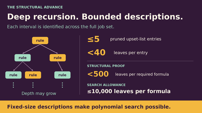
Each candidate job set is described using Boolean combinations of atomic tests: membership in a named triple, precedence to or from that triple, and rank thresholds in the chosen order or its reverse. A formula leaf is one atomic test or its negation.
The crucial distinction is global versus local agreement. A predicate may select the correct jobs inside a known interval while also selecting unrelated jobs elsewhere. A reusable subproblem needs a description correct on the entire padded job set. Repeatedly intersecting ancestor predicates would solve that locality problem only by accumulating unbounded history.
Instead, the proof carries short lists of global upsets. An upset is closed under successors: once it contains a job, it contains every later precedence successor in the current direction. On the current interval, the list selects precisely the high jobs. Rank thresholds trim inherited entries, and entries selecting nothing in a child are pruned.
Why can only five entries survive? At most two entries initialize a direction run. Each additional surviving injection contains a high child job with a successor in the child’s ending triple. Upset closure puts that successor in the same injection. The injections are disjoint on the parent, forcing distinct witnesses. Three boundary jobs can support at most three such injections.
Boundary invariants handle the missing global control. One excludes distant qualifying jobs unless the boundary’s predecessor cone accounts for them. Another prohibits specified improving exchanges even after any feasible child reordering. When direction changes, paired inherited entries can be flattened locally, then combined with boundary tests to obtain a globally valid short description.
| Object | Established Bound | Role |
|---|---|---|
| Pruned upset list | At most five entries | Limits inherited components. |
| Each entry | Fewer than 40 leaves | Limits each component’s formula. |
| Required descriptions | Fewer than 500 leaves | Covers global nodes and relative splits. |
| Enumerated family | At most 10,000 leaves per formula | Fixed search allowance, independent of input size. |
The final global tests first use positive predecessor and successor cones to locate a candidate inside a parent domain. Only there do they apply a cutoff description known to agree locally. Additional weak-cone exclusions remove boundary jobs and jobs beyond the gap. That order prevents a locally correct simplification from silently importing exterior jobs. The final formulas therefore describe actual child sets across all jobs, without appending every ancestor’s membership test.
The advance is this persistent bound through recursive decomposition. Recursion may be deep. Its descriptions stay small, allowing a polynomial family to contain every subproblem the proof needs. This is a structural compression theorem, not an assumption that only a few schedules exist.
9. How Dynamic Programming Reconstructs the Optimal Schedule
Enumerate the bounded-description family and represent each distinct set by an -bit membership vector. Process sets in increasing cardinality. Accept the empty set and reject sets whose size is not divisible by three.
For a remaining set , consider states . Here is an antichain triple, is the earlier part, and the later part. They partition . In this section, names a job set, not the binary input length used in the runtime theorem.
The earlier part must itself have a bounded relative description within the current set. This restricts state enumeration to the fixed formula family. Accepted gaps must also belong to that family. The structural theorem proves these restrictions retain at least one successful decomposition whenever a feasible schedule exists. Without that completeness argument, restricting the table would merely be a heuristic that might discard the optimum.
Keep only compatible states, with no precedence pointing backward between their parts. A state is initial when its left set was accepted, and final when its right set was accepted. A transition advances to another marked triple when the already covered jobs remain covered and the intervening gap was accepted.
An initial-to-final path concatenates accepted smaller gaps and marked triples into a full schedule. This proves soundness. Completeness uses the bounded-description hierarchy: every feasible instance has marks and child intervals inside the enumerated family, so the dynamic program can find an accepting path.
Store predecessor records and schedules to reconstruct the answer. Test deadlines from one through the original job count, choose the smallest feasible deadline, and delete dummies. A topological ordering always permits a sequential schedule within that range. The search therefore terminates with the exact optimum.
10. Why the Algorithm Is Polynomial-Time but Not Practically Fast
The search fixes formula leaves. There are atomic tests, so assigning tests to a fixed-size formula gives possibilities, up to a constant depending on . This is polynomial because never grows with the input.
The full implementation also accounts for state pairs, table scans, copying, reconstruction, and deadline trials. That conservative accounting yields exponent 150020. It is an upper bound, not a claim that every instance requires exactly that many operations.
An exponent this large makes “polynomial” a complexity classification rather than an engineering recommendation. Compare the still-exponential improvement in our Subset Sum analysis: classification and usable performance answer different questions. Likewise, edit distance approximation offers a different accuracy-runtime contract.
For developers, applying the theorem starts with checking whether a workload matches its assumptions. Different task durations, data-transfer delays, or constrained worker types change the mathematical instance. Encoding such a system as a unit-job DAG without justification could make the returned optimum irrelevant to the actual workload.
The paper supplies no benchmark showing this method beats existing schedulers. Its practical research value is a structural route that future algorithms might simplify, with smaller descriptions or a less exhaustive search.
11. Lean Verification, Theorem Limitations, and What Remains Open
OpenAI included the result in its mathematics release. The Lean scope note covers exact optimization, deadline feasibility, and a fixed finite machine with polynomial runtime. The comparator configuration points to a separate implementation proof. The comparator’s placeholder is a target statement, not that implementation. We have not independently rebuilt the formalization.
Published formal checking evidence differs from independent peer review, a distinction explored in our Lean formalization explainer. The theorem also does not extend automatically to four machines, unequal durations, communication costs, or additional resources.
A fixed three-machine result leaves other fixed machine counts beyond its scope. Allowing machine count as input gives a known NP-complete problem, so this does not establish P equals NP. Input and resource models matter, as in our Turing-machine tradeoff coverage.
The useful next question is how much of the bounded-description structure survives in a substantially faster algorithm. For three machine scheduling, the proof supplies an exact theoretical solution and a concrete mechanism to improve. Follow Binary Verse AI for research explainers that trace the argument from assumptions to algorithm, including what remains untested.
What exactly did OpenAI solve in three-machine scheduling?
The proof establishes a uniform deterministic polynomial-time algorithm for nonempty collections of nonpreemptive unit-length jobs with arbitrary acyclic precedence constraints on three identical parallel machines. It decides deadline feasibility and constructs a schedule with minimum makespan.
Why was three-machine scheduling difficult when two machines were already solved?
The extra machine creates packing choices that earlier two-machine structural arguments did not resolve. Polynomial algorithms for two processors and restricted precedence graphs did not establish a general exact solution for three machines.
What was the best approach before OpenAI’s proof?
Earlier work included exact algorithms for restricted precedence structures and approximation schemes. Nederlof, Swennenhuis, and Węgrzycki’s SODA 2025 result provided a general exact subexponential-time algorithm for fixed machine count, including three. It did not provide polynomial time.
How does the OpenAI proof avoid exponentially many scheduling possibilities?
It proves that a suitable recursive decomposition has globally valid, bounded-size descriptions of interval job sets, together with bounded relative descriptions of marked splits. A dynamic program searches a polynomial-size family containing the required subproblems, rather than enumerating every schedule.
Does the algorithm guarantee the shortest possible schedule?
Yes, within the stated model. It decides whether each candidate deadline is feasible, selects the smallest feasible deadline, and reconstructs a schedule achieving it. The schedule therefore has minimum makespan.
Why is an algorithm with exponent 150020 considered polynomial-time?
The exponent is a constant independent of input size. The stated bound is therefore polynomial in binary input length, although it is far too large to establish practical efficiency. The paper reports no competitive scheduling benchmark.
Has the three-machine scheduling proof been formally verified?
OpenAI has published a Lean formalization whose stated scope includes the exact scheduling theorem and a fixed finite machine with polynomial runtime. Its comparator configuration points to a separate implementation proof. We have not independently rebuilt it, and formal-checking evidence should not be described as independent peer review.