
A graph can demand many colors while refusing to collapse into an equally large complete graph. OpenAI’s September 23, 2026 manuscript constructs precisely that separation, presenting a disproof of the Hadwiger Conjecture, proposed in 1943. Its counterexamples have no independent set larger than two vertices, yet their largest clique minors fall well below the resulting coloring requirement.
The research manuscript presents arbitrarily large finite examples. The repository publishes an ordinary-counterexample Lean formalization, with a narrower scope than the paper’s additional fractional-coloring consequence. This article explains the argument and that verification boundary. The surprise is architectural: an elementary parity contradiction controls coloring, while a much longer probability argument prevents the contractions that Hadwiger’s prediction requires.
Table of Contents
1. What Is Hadwiger’s Conjecture in Graph Theory?
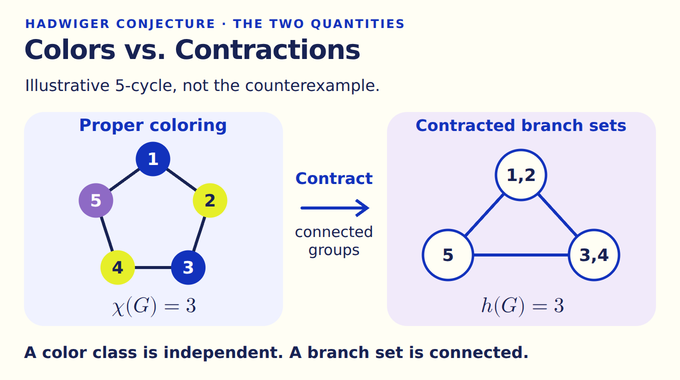
A proper graph coloring assigns different colors to adjacent vertices. The chromatic number is the minimum number needed. Think of scheduling incompatible jobs: each color is a time slot, and an edge forbids sharing it.
The Hadwiger number measures something different: the largest complete graph obtainable as a minor through vertex deletions, edge deletions, and edge contractions. Equivalently, choose disjoint connected branch sets, with an edge joining every pair. Contract each branch set to one vertex.
That was the conjectured universal inequality. Hadwiger number versus chromatic number compares a compression structure with a coloring constraint. Neither number merely counts the original graph’s largest clique.
| Item | Verified Manuscript Statement |
|---|---|
| Original prediction | Every finite nonempty simple graph satisfies . |
| Main construction | Arbitrarily large orders , with and . |
| Resulting separation | For , . |
| Verification boundary | Published Lean scope covers the ordinary counterexample, excluding the fractional strengthening. |
This concerns finite abstract graphs. The Hadwiger–Nelson problem instead colors points of the Euclidean plane subject to a distance rule. Their shared surname does not make their theorems interchangeable.
2. Why Hadwiger’s Conjecture Survived for 83 Years
In the formulation “excluding a minor permits colors,” the cases were established. Wagner connected the case to the Four-Color Theorem. Robertson, Seymour, and Thomas proved the next case: graphs without a minor are five-colorable. These remain valid.
Beyond those cases, approximate bounds improved without reaching the conjectured coefficient. The manuscript traces a progression from colors for graphs excluding to , and cites a recent preprint reaching . An asymptotic bound still allows a gap from the exact prediction.
Independence-two graphs sharpened the challenge. Their color classes contain at most two vertices, so a graph on vertices requires at least colors. Earlier general results guaranteed roughly branch sets, with improvements below a linear extra term. The unresolved distance between one-third and one-half was substantial. Unlike the planar Hamiltonian-cycle question in Barnette’s conjecture, this construction has no planarity restriction.
3. OpenAI’s Hadwiger Conjecture Counterexample: The Main Theorem
Theorem 1.1 targets two quantities simultaneously: the independence number , the largest independent-set size, and the connected-matching number .
A matching is a collection of vertex-disjoint edges. Here “connected matching” means every pair of matching edges touches: at least one edge joins their endpoint sets. Merely belonging to the same connected component is insufficient.
The objective is therefore demanding. Every triple must contain an edge, keeping independent sets small, but sufficiently large matchings must contain two edges with no contact whatsoever. The proof achieves this by designing the absent edges first. Such an absent edge is called a hole. The final graph connects precisely the distinct sampled positions whose configurations have no hole between them.
This reverses the usual intuition about density. Adding edges makes coloring harder, but it can also create the contacts needed for a complete minor. The construction must preserve enough missing edges to obstruct contractions without leaving any independent triple. An arbitrary dense random graph does not automatically deliver that carefully balanced combination.
4. How the Proof Constructs a Triangle-Free Relation of Missing Edges
Work over , the field with two elements, where addition is parity. Let be a coefficient space, a linear functional, and a symmetric bilinear form. The affine-gradient map is . It turns a vector into a linear functional.
Each configuration carries an injective map into a shared space and a functional on that space. A hole requires witnesses satisfying four conditions:
The first equality gives the witnesses a common image. Their -values disagree. The other identities constrain whole functionals, so checking one vector would not suffice. This algebraic certificate will forbid a triangle of holes while leaving room for four-hole conflicts.
For developers, a witness is comparable to a certificate accepted by an exact checker. The graph’s nonadjacency rule asks whether suitable witnesses exist. That analogy explains what the equations do, but implies no efficient search procedure for finding them. The shared ambient space lets certificates at different vertices interact, which is essential for the contradiction.
5. Why Three Missing Edges Force a Contradiction Over the Binary Field
Assume three configurations have holes on all three pairs. Write for the witness at endpoint of the hole joining and . Evaluate each relevant functional identity on the witness toward the third vertex, then sum over all six ordered triples.
The shared-image conditions make the left-hand terms cancel in pairs. Symmetry makes the bilinear terms cancel too. Each undirected hole contributes one remaining parity bit, giving:
That is impossible in . Lemma 2.2 therefore excludes hole triangles. Injectivity also excludes a hole from a configuration to itself.
An independent triple in the final graph would require exactly such a triangle of holes. Consequently holds deterministically. Even repeated sampled configurations cause no difficulty: distinct positions carrying the same configuration are adjacent. This resolves the coloring side before any probabilistic estimate begins. It does not yet control clique minors.
6. Boolean Moment Matrices, Cut Profiles, and Tensor Frames
The abstract certificate needs a concrete realization rich enough to force conflicts. The construction evaluates selected monomials at Boolean points, collecting them into a vector . Its point moment is a rank-one matrix encoding products of those evaluations.
Tags allow different variable blocks. For each tag, the allowed moments span a space. A cut profile records pairwise sums of moment choices across tags. Those sums act like differences because the arithmetic has characteristic two. This organizes shared information while controlling ambiguity between representations.
Injective frame maps embed these coefficient directions into common binary spaces. Prescribed Gram matrices, which record pairings between frame columns, make those embeddings respect the required algebra. Auxiliary columns supply freedom for later cross-contraction equations.
The resulting tensor map remains injective, and its companion functional satisfies . The hole relation now lives on a finite probability space of frames. Rank-one matrices also appear in our Borsuk counterexample explainer, but here they encode Boolean algebra rather than Euclidean distances.
The parameter order matters. Most budgets and dimensions are fixed before the growing parameter tends to infinity. Mixer maps are chosen before the candidate unit distribution is considered. Otherwise the construction could silently adapt to each attempted matching, proving a weaker statement than the uniform obstruction needed for a single graph.
7. The Four-Hole Obstruction That Destroys Connected Matchings
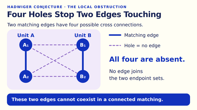
An ordered pair without an internal hole is a unit, representing a possible matching edge. Consider two disjoint units, with endpoints and . If every cross pair is a hole, no edge joins the units. They cannot coexist in a connected matching.
Notice the compatible shapes: a four-cycle of holes is allowed even though a triangle of holes is forbidden. This distinction makes the entire construction possible.
The witnesses for the four cross holes are short sums of point moments. Paired lists match corresponding points across units. A point’s key records its images under the relevant frame maps. Equal keys yield the shared tensors required by the hole equations.
A scalar recipe additionally prescribes parity and pairing conditions needed for the functional identities. Pins retain selected frame images during conditioning. Proposition 7.1, the key-collision criterion, converts sufficient overlap between accepted key distributions into a lower bound on four-hole probability. Collision alone is insufficient unless the acceptance conditions also survive.
The proof keeps the mass lost to acceptance tests in its probability bookkeeping. Renormalizing every successful query to total mass one would conceal how rarely its certificates occur. These unnormalized distributions preserve the actual probability cost when the algebraic realization is transferred back to independently drawn units.
8. How Supersaturation Forces Four-Hole Conflicts
Theorem 3.1 is the analytical core. Supersaturation here means that every sufficiently spread-out unit law must contain a quantified probability of conflict. Let denote the raw frame distribution and a distribution on units. Both endpoint marginals must be bounded by a fixed multiple of , and the joint law must be bounded by . These pointwise caps prevent excessive concentration.
Under those assumptions, two independent units have four cross holes with probability at least . Here is the ambient dimension, while and are fixed construction constants. Endpoints within one unit may remain dependent, as matching edges require.
The proof conditions on exact pin images, partitioning the law into leaves. Phase estimates prepare compatible pairing tables. Mixed-law estimates and Fourier bounds control key tests across those leaves. Boolean Fourier analysis is also a tool in the Courtade–Kumar research, although the desired inequality here is different.
Weak product comparison transfers single-key control to permitted tests of full key tuples. Two overlap regimes need separate arguments: positive limiting compatibility mass uses a common limit and finite-dimensional duality to find a feasible scalar recipe. Compatibility mass of order can vanish in that limit. A uniform large-set estimate handles that regime separately, selecting a bounded family of sets on one leaf before sampling the opposite leaf.
The endpoint dependence is a major technical obstacle. A matching chooses edges using information about both endpoints, so treating those endpoints as independent would discard the very families that must be ruled out. The mixed-law and product estimates retain the permitted dependencies and pairing constraints. Their conclusions concern specified tests, rather than an unrestricted claim that every conditioned distribution becomes random.
9. How Entropy Containers and Random Sampling Produce the Counterexample
A matching in the sampled graph need not obey the distributional caps directly. The proof bridges that gap with a conflict graph whose vertices are units. Four-hole pairs are adjacent, so a connected matching supplies an independent family of units.
While a residual family supports an admissible law, choose one minimizing relative entropy against . Supersaturation supplies a substantial conflict neighborhood. Record selected members of the independent family and remove their neighborhoods. Each recorded deletion that leaves an admissible law raises the minimum feasible entropy, bounding the fingerprint length.
When no admissible law remains, a capacitated cut covers the residual family using a small set of endpoint types and a small set of exceptional pairs. The random sample simultaneously keeps both exceptions too small to support a matching of size .
A fingerprint is a compressed record of the deletion process. Deterministic choices let the argument reconstruct the terminal family from that record. There are few enough records, relative to the enormous sample, to apply a union bound over all of them. This is how a probability estimate for each admissible law becomes control over every connected matching at once.
Proposition 3.4 gives success probability at the prescribed orders , for sufficiently large parameters. This is an asymptotic existence argument with enormous fixed constants. It supplies no demonstrated efficient generator or practical graph-coloring speedup. The smallest counterexample and computationally manageable witness sizes are not established by this construction.
10. From Connected Matchings to the Final Clique-Minor Inequality
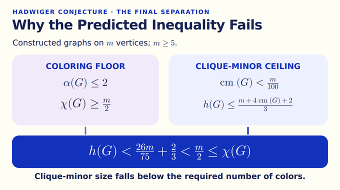
The final step is elementary counting. In a complete-minor model with branch sets, let be singletons and have two vertices. Write .
Every two-vertex branch is an edge. The singletons form a clique, so pairing them contributes another edges. Together these form a connected matching. Hence , implying .
| Branch Type | Count | Vertices Used |
|---|---|---|
| Singleton | ||
| Two vertices | ||
| At least three vertices | At least |
Adding the vertex costs yields . Substituting the bound on gives . Maximizing over models proves Proposition 3.5:
Insert . For , the result is:
This is the Hadwiger conjecture counterexample: the minor ceiling lies below the coloring floor. No exact chromatic number or exact largest minor needs to be computed.
The counting argument also explains why connected matchings are the right intermediate object. Many small branch sets would manufacture a large touching matching. If small branches are scarce, the remaining branches each consume at least three vertices, limiting how many fit. Either way, a large complete minor becomes impossible under the theorem’s matching bound.
11. What OpenAI’s Proof Establishes and What Remains Unresolved
Fractional coloring assigns nonnegative weights to independent sets, covering each vertex with total weight at least one. Summing coverage constraints gives . Thus the paper also obtains:
This refutes the fractional Hadwiger conjecture discussed by Reed and Seymour. Only coloring is fractional here. The minor number remains ordinary.
Fractional weights cannot evade the obstruction because every independent set still covers at most two vertices. Allowing partial use of many such sets changes the optimization problem, but cannot reduce its total cost below half the vertex count. The same minor upper bound therefore defeats this relaxation without requiring a second graph construction.
The published Lean scope note covers arbitrarily large ordinary counterexamples and the quantitative inequality. The implementation module contains proof bodies for those existence and contradiction theorems. The fractional strengthening and Colin de Verdière consequence lie outside the selected statement. Binary Verse AI has not independently rebuilt that development. As our coverage of AI mathematical proofs and formalized percolation research emphasizes, published formalization and independent reproduction are distinct evidence.
OpenAI included this work in its October mathematics release. That release establishes provenance, not a paper-specific performance benchmark. The constructive lesson for researchers is the separation between deterministic local certificates and distributional global obstructions.
One weaker question survives: must independence-two graphs always have connected matchings of some positive linear size? A counterexample below one-hundredth does not exclude a smaller universal coefficient. The Hadwiger Conjecture story therefore ends with a precise failure and a sharper next question. Follow Binary Verse AI for research explanations that trace the proof, its verification scope, and the problems it leaves open.
Has Hadwiger’s conjecture been disproved?
OpenAI’s September 2026 manuscript presents arbitrarily large finite graphs satisfying , which disproves the conjecture if the argument is correct. The repository publishes a Lean formalization of the ordinary counterexample. That published artifact should be distinguished from an independently reproduced check or established expert consensus.
What is the difference between a graph’s chromatic number and Hadwiger number?
The chromatic number is the fewest colors needed to give adjacent vertices different colors. The Hadwiger number is the largest obtainable as a minor through vertex deletions, edge deletions, and edge contractions. A clique minor may use connected groups of vertices rather than single vertices.
Why does OpenAI’s counterexample use graphs with independence number two?
When , every color class contains at most two vertices. An -vertex graph therefore requires at least colors. The construction keeps clique minors below , producing a contradiction to Hadwiger’s predicted inequality without computing the exact chromatic number.
How does the new proof prevent large complete graph minors?
The construction forces missing-edge patterns that obstruct large connected matchings. The manuscript proves and the general bound . Here a connected matching requires every pair of matching edges to touch. Combining the bounds places the Hadwiger number below the coloring requirement.
Why are four missing cross edges important to the proof?
Two disjoint matching edges have four possible cross edges between their endpoint sets. If all four are missing, the matching edges do not touch and cannot belong to one connected matching. The proof forces these conflicts under specified distributional density bounds, then transfers the obstruction to sampled finite graphs.
Does OpenAI’s proof also disprove the fractional Hadwiger conjecture?
The manuscript also proves examples satisfying , refuting the fractional-coloring weakening discussed by Reed and Seymour. The clique-minor number remains ordinary. This strengthening is outside the selected ordinary-counterexample Lean statement described in the repository’s scope note.
Does the counterexample contradict the Four-Color Theorem or the Hadwiger–Nelson problem?
No. The Four-Color Theorem and established low-order cases of Hadwiger’s conjecture remain valid. The Hadwiger–Nelson problem colors points of the Euclidean plane subject to unit-distance constraints. It is a separate mathematical question.