
Imagine stepping from prime to prime across the complex plane, always keeping the next jump below the same fixed limit. OpenAI’s September 26, 2026 manuscript answers that challenge negatively: the Gaussian moat conjecture admits no infinite walk through distinct Gaussian primes with bounded steps. Its stronger conclusion caps every connected component, wherever the walk starts. The surprise is how it gets there. Geometry supplies differences, arithmetic separates them, and information theory shows that avoiding composite points would demand more information than bounded movements can carry.
Table of Contents
1. Gaussian Moat Conjecture Solved: What Exactly Did OpenAI Prove?
Bounded-Step Walks on Gaussian Primes states a proof of the uniform Gaussian moat conjecture. For each finite real step bound , one finite number bounds all components of the Gaussian prime graph. The manuscript belongs to OpenAI’s October mathematics release, attributed to an internal frontier model.
1.1. Gaussian Moat Conjecture: Key Facts
| Research Detail | What the Manuscript Establishes |
|---|---|
| Manuscript date | September 26, 2026. The paper is authored by OpenAI. |
| Main conclusion | Every fixed finite step bound has a uniform finite component-size bound, independent of the starting Gaussian prime. |
| Walk restriction | Visited Gaussian primes must be distinct. Distance is Euclidean, and the step bound stays fixed. |
| Scope | All Gaussian primes, including coordinate-axis primes and their associates, are covered. |
| Proof mechanism | A finite periodic sieve, geometric sampling, residue coverage, and an entropy-budget contradiction. |
| Quantitative limitation | The bound exists but no explicit function of the step allowance is supplied. |
“Fixed” matters. You may choose an enormous jump allowance before starting, but cannot keep increasing it indefinitely. The conclusion concerns distinct visited primes. Repeatedly shuttling between two nearby primes is no counterexample. The theorem is stronger than saying that each particular starting point eventually traps you.
2. What Are Gaussian Primes, and How Can You Walk Between Them?
Gaussian integers form , with . Their norm is , and Euclidean length is . A Gaussian prime is irreducible: any factorization has a unit factor, one of .
For example, is prime because its norm is the ordinary prime . The integer is also Gaussian prime, despite having norm . By contrast, is reducible. Ordinary primes congruent to modulo split into conjugate factors. Those congruent to remain irreducible, while ramifies.
A legal short walk is . Its jumps have lengths and , so permits both. All three vertices are prime and distinct. Distance, rather than the difference between their norms, determines legality.
3. The Original 1962 Gaussian Moat Problem: Can a Prime Walk Continue Forever?
The manuscript traces the question to Basil Gordon at the 1962 International Congress of Mathematicians. Erdős later credited Gordon and Motzkin, recalling a conversation with Motzkin in 1963. That history explains the 64-year framing.
Define by joining distinct Gaussian primes whose distance is at most . A self-avoiding walk never revisits a vertex. The question asks whether some fixed permits an infinite such walk.
On the ordinary prime number line, a sufficiently long composite interval blocks progress outright. In two dimensions, sideways escape remains possible. The connectivity language resembles percolation theory, but this graph is determined by arithmetic. Its vertices are not independently retained at random.
4. Why Previous Attempts Could Not Prove the Gaussian Moat Conjecture
Earlier work constructed arbitrarily large prime-free disks and arbitrarily isolated real Gaussian primes. These are genuine obstructions, but an empty disk is a lake, not necessarily a coastline extending across every possible route.
Tsuchimura’s computation bounded the region reachable with jumps of length at most six from the origin, added as an initial vertex. That controls one component, not every starting prime for every bound.
Gethner and Stark established periodic obstructions for step bounds and , while Vardi studied periodic coprimality graphs and uniform component bounds. The missing ingredient was a finite collection of congruence restrictions that works for every fixed . Searching farther from one origin could not supply that universal quantifier.
5. Theorem 1.1: Why Every Gaussian Prime Component Has a Uniform Finite Bound
In mathematical form, the main assertion is:
Here counts vertices. The same works for every starting prime, including axis primes and all associates, meaning multiplication by a unit. Consequently, every injective bounded-step walk has at most terms, hence at most steps.
This uniformity is substantial. A graph can have finite components of sizes one, two, three, and so on without any infinite component. The theorem excludes that possibility here. For , distinct lattice points cannot be adjacent, so suffices. For larger bounds, the argument establishes existence without providing a numerical estimate.
6. The Finite Sieve Obstruction: How OpenAI Restricts Every Possible Walk
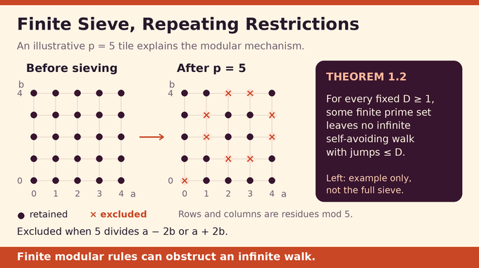
Choose finitely many ordinary primes , each splitting as . Reduction modulo either Gaussian factor gives a field with elements. These residue fields are related to the algebra discussed in our prime-field factorization explainer.
For a finite selection , define the avoiding set:
Theorem 1.2 supplies one finite set , depending only on , whose avoiding set contains no infinite self-avoiding bounded-step lattice walk. Importantly, the surviving points need not themselves be prime. Blocking this larger set blocks prime walks too, apart from finitely many exceptions.
That finite sieve obstruction is the real engine. The proof must establish that suitable primes exist uniformly over all hypothetical walks. Choosing different restrictions after seeing each walk would not establish the theorem.
7. Why Periodicity Converts the Sieve Into a Uniform Component Bound
Put . Translating by either coordinate multiple of preserves the avoiding set. This is the repeating-cell idea familiar from periodic lattice tilings.
Each vertex has finitely many bounded-length neighbors. An infinite component would therefore contain an infinite simple path, by the finitely branching tree of finite paths. The sieve theorem rules that out.
Now suppose two points in one finite component agree modulo in both coordinates. Translating by their nonzero difference maps that component onto itself. Repeating the translation would produce infinitely many points, a contradiction. Each component therefore injects into the residue cells.
Let contain the associates of the selected Gaussian factors, and let count lattice vectors of length at most , including zero. Deleting puts every remaining Gaussian prime inside the avoiding graph. Restoring those exceptions gives Proposition 2.1:
Only finitely many pieces can attach to the exceptional primes. This transfers the sieve’s bound to the entire prime graph.
8. Torus Geometry: How Long Walks Generate Enough Distinct Differences
To prove the sieve exists, fix any deterministic infinite self-avoiding lattice walk. For a segment of steps, temporarily use for its visited points. Let be its diameter and its greatest distance from a diameter line, increased to at least one. Set .
Lemma 4.1 establishes:
Here contains distinct displacement vectors, and the positive constants have the dependencies indicated by their subscripts. Packing disjoint small disks around visited lattice points proves the first lower bound.
The difference bound needs topology. When , diameter endpoints and a farthest point generate a lattice of area . Subtract two interpolated walk paths modulo that lattice. The resulting torus map has degree minus one, so it must cover the target torus. Every image lies within of a vertex difference. Disks around those differences must therefore cover area .
The sampling rule chooses a distinct difference uniformly, selects a representative endpoint pair, then flips a coin between its endpoints. Uniformly sampling pairs instead would overweight frequently repeated differences.
9. Random Signed Prime Factors and the Growth of Residue Entropy
For each selected split prime, choose one conjugate factor with a fair coin. “Signed” refers to that choice. The walk remains deterministic. Randomness belongs to the proof’s measurements.
Lemma 4.2 controls collisions after reduction modulo products of chosen factors. If nearby sign choices have witnesses in a sufficiently small rectangle, common divisors force their determinant to be divisible by a number larger than its possible nonzero magnitude. The witnesses must be collinear.
More precisely, write for distinct split primes in , with . For a rectangle with half-lengths satisfying , where , the probability of a nonzero multiple of the signed product inside it is at most , provided is sufficiently large. That turns geometric separation into a quantitative arithmetic estimate.
For a fixed direction, Hoeffding concentration makes such a witness unlikely. Expansion in the Boolean cube of sign choices then controls all directions together: distinct direction classes have disjoint enlarged neighborhoods. This avoids an uncontrolled count of possible lines.
Define as the average joint residue entropy of a sampled position over signed subsets of size . All logarithms are natural. With the batch’s mean logarithmic prime size, suitable input and output sizes satisfy Lemma 4.3:
Repeated enrichment halves the entropy deficit up to controlled error. Entropy is a rigorous uncertainty measure, as in the Courtade–Kumar information problem, rather than a synonym for visual disorder.
The sizes are and , with segment length . Large scales and small make the errors controllable while matching consecutive sampling operations.
For probabilities , entropy is , with zero-probability terms contributing zero. A uniform variable with possible values has entropy . Conditional mutual information, , measures how much learning reduces uncertainty about after is already known.
10. From High Entropy to Residue Coverage: The Proof’s Critical Bridge
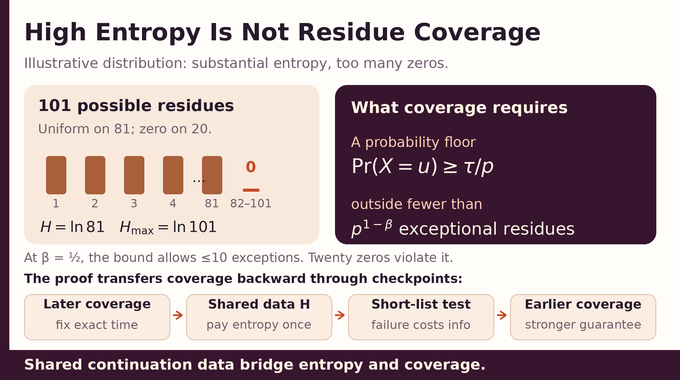
High joint entropy does not ensure that each residue gets useful probability. A distribution can have nearly maximal entropy while entirely omitting some symbols. The needed coverage statement is:
Thus almost every residue has probability at least , with an explicitly controlled exceptional set. The proof obtains this by transferring coverage backward through checkpoints, although every sampled walk time moves forward.
Fix an exact later checkpoint. Run independent continuations from it, recording their displacements together in one data vector . If terminal coverage fails, candidate starting residues can be tested against the deficient set. The true residue lands on a short candidate list with appreciable probability. Coverage from that exact checkpoint makes most false candidates unlikely to survive repeated trials.
The short-list inequality then forces a conditional entropy deficit. But high joint entropy and the small entropy of cannot support such deficits across many coordinates. Crucially, the shared displacement vector is charged once, not separately for every residue.
The quantitative principle is simple. If an alphabet has size and data identify a list of size at most containing the true value with probability , then:
Here is binary entropy and is the observed data. A short successful list reveals information even when success depends on the hidden value. Independence is required for repeated continuations only after fixing their exact checkpoint, not before that conditioning.
10.1. What the Sampling Schedule Supplies
| Stage | Mathematical Job |
|---|---|
| Top band | Build joint residue entropy of order for the batch of primes near , and preserve it through later stages. |
| Middle band | Use exact checkpoints and inexpensive shared continuation data to transfer the required coverage backward. |
| Bottom band | Obtain exceptionally accurate one-coordinate entropy to start the backward coverage induction. |
| Final smoothing | Add an independent uniform time offset so every prime batch uses one terminal law that changes little under short time shifts. |
The schedule uses decreasing geometric scales in widely separated windows. Later movements have small displacement entropy compared with information accumulated earlier. An independent uniform time offset makes the common terminal law nearly invariant under the short shifts used in block comparisons. No stationarity assumption is imposed on the original walk.
At the initial checkpoint, at least 99% of signed factors receive terminal coverage with probability floor outside fewer than residues. These are auxiliary sampling guarantees, not measured properties of randomly generated prime walks.
11. The Final Contradiction: Why Zero Avoidance Costs More Information Than a Walk Can Carry
Assume the walk avoids every selected zero class. A short increment word tests candidate starting residues: a candidate is impossible if its translated word hits zero. Self-avoidance makes the hit opportunities disjoint when , since a nonzero multiple of a factor of norm has length at least .
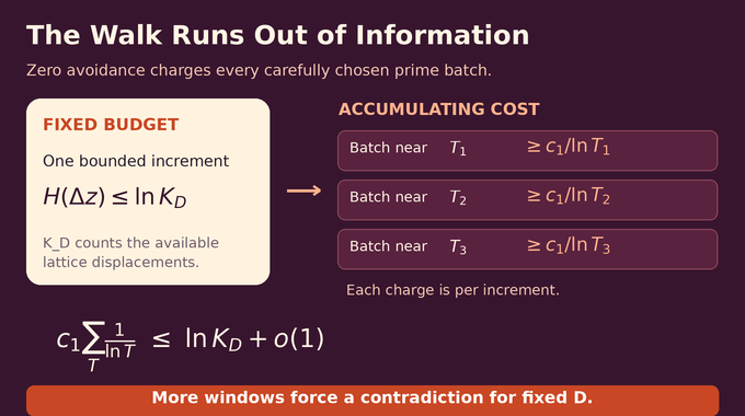
Coverage therefore makes repeated tests eliminate most candidates. The manuscript uses dyadic lengths comparable to for primes near . After accounting for displacement entropy, Proposition 7.1 charges conditional mutual information of at least per increment to each batch.
Let be that batch’s terminal residue vector and contain earlier batches. Write for the conditional mutual information , averaged over auxiliary choices. Nested residue vectors, dyadic block subadditivity, and smoothing yield:
Here is the increment word, records auxiliary prime choices, and tends to zero as the schedule grows. The paper connects this budgeting method to Tao’s entropy-decrement argument, also relevant background to the two-point Chowla story.
Each increment has only possible values. Yet the selected prime windows force:
Each window contributes a fixed positive amount, and the number of windows grows without bound. The right side stays finite. Uniformity over walks lets the proof choose one sufficiently large finite schedule, giving , then Theorem 1.1 through periodicity.
Why does a window contribute enough? Its logarithmic width grows in proportion to its location. Geometrically spaced batches therefore supply proportionally more terms, each proportionally smaller. Their aggregate stays bounded below rather than disappearing as the primes become enormous.
The bound remains nonexplicit. This is not a practical maximum-walk calculator. Developers can illustrate finite components, but a large simulation cannot replace the uniform argument.
The official Lean scope reports formalization of the no-infinite-walk result and uniform component bound, including axis primes and associates. That concerns the encoded theorem, not separate verification of every paragraph of the 29-page exposition. We did not rebuild the Lean project. The distinction between discovery and formalization also guides our Fermat proof explainer.
The Gaussian moat conjecture’s resolution turns a local jump restriction into a global information contradiction. For more explanations that follow the actual mathematical mechanism, explore Binary Verse AI’s AI mathematical proofs coverage and follow the research series.
12. Gaussian Moat Conjecture: Frequently Asked Questions
Has the Gaussian moat conjecture been solved?
OpenAI’s September 26, 2026 manuscript presents a proof that no infinite sequence of distinct Gaussian primes can maintain a fixed finite maximum step length. It states the stronger result that every connected component has a uniform finite size bound depending only on that step limit. OpenAI lists the main result as formalized in Lean.
What is a Gaussian prime? Can you give an example?
A Gaussian prime is an irreducible element of . For example, is prime because its norm is , an ordinary prime. However, itself is not Gaussian prime, because . The ordinary integer is Gaussian prime even though its norm is .
Why didn’t large prime-free regions already prove the Gaussian moat conjecture?
A prime-free region blocks a local route, but a walk in the two-dimensional Gaussian integer lattice may go around it. The challenge was to rule out every infinite bounded-step route, rather than merely construct arbitrarily large empty regions.
Does OpenAI’s proof calculate the maximum number of Gaussian primes in a bounded-step walk?
It proves that a finite bound exists for every fixed step limit , independently of the starting prime. The proof is nonexplicit: it does not give a numerical formula or usable estimate for that bound. It also does not identify the exact largest achievable walk.
Why does the proof use entropy and information theory?
The proof measures uncertainty in residues of sampled walk positions. Avoiding selected zero residues forces short increment sequences to reveal information about their starting positions across many prime batches. Those information costs eventually exceed the finite per-increment entropy budget, producing a contradiction.
Does the result include Gaussian primes on the coordinate axes?
Yes. The uniform component bound covers coordinate-axis primes and all associates. When passing from the periodic avoiding graph to the full Gaussian-prime graph, the proof restores the finitely many associates of the selected Gaussian factors and bounds the additional components that they can connect.
Is OpenAI’s Gaussian moat proof formally verified in Lean?
OpenAI’s official scope note reports a Lean formalization covering every real step bound, all starting Gaussian primes, and the uniform component-size conclusion. This describes formalization of the stated result, not separate formal verification of every line of the 29-page exposition. Binary Verse AI did not independently rebuild the Lean project.