

A phase transition can be known to exist while its most distinctive prediction remains unproved. That was the gap facing the BKT transition in the original square-lattice XY model: exactly how fast does the distance over which spins remain correlated grow near criticality?
OpenAI’s October 5, 2026 preprint proves that the logarithm of this correlation length, multiplied by the square root of the distance to critical inverse temperature, approaches one finite, strictly positive constant. The result establishes the predicted essential singularity for the nearest-neighbor cosine interaction. Earlier rigorous work established the transition, but this precise asymptotic required two additional bridges: controlling how temperature crosses the critical renormalization trajectory and identifying the resulting scale with physical spin correlations.
Table of Contents
1. BKT Transition: What OpenAI’s Proof Actually Establishes
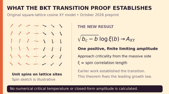
Theorem 1.1 in the original research paper states:
Here is inverse temperature, its critical value, and the axis correlation length in lattice units. The approach is from , the hotter, massive phase. “Massive” means correlations have a positive exponential decay rate.
| Research Detail | Verified Scope |
|---|---|
| Microscopic Model | Nearest-neighbor cosine XY interaction on the square lattice. |
| Main Result | A single positive, finite limiting amplitude for the logarithmic correlation-length divergence. |
| Limit Convention | Free-box thermodynamic limit first, axis separation limit second. |
| Dependencies | Two companion preprints supply critical height and analytic-map inputs. |
| Publication Status | October 2026 research preprint; peer review and full formal verification are not established here. |
Equivalently, . The vanishing error belongs inside the exponent when exponentiating. The theorem does not supply a constant multiplicative prefactor for the correlation length. Its amplitude also depends on the interaction’s normalization.
The single limit is stronger than proving only that the logarithm stays between two positive multiples of the inverse square root. Such bounds identify a growth scale but leave room for persistent variation in its leading coefficient. The theorem rules out that variation for this model and this definition of mass.
2. The Original Problem: The BKT Transition In The 2D Cosine XY Model
Place a unit arrow at each site of the integer square lattice. Its angle is , understood modulo . On a finite box with free boundaries, a configuration receives Boltzmann weight proportional to:
The edge set counts each unordered neighboring pair once and contains no exterior bonds. Positive favors alignment. Increasing inverse temperature cools the system, which is easy to reverse accidentally when reading the theorem.
The Berezinskii–Kosterlitz–Thouless transition separates exponential decay from a low-temperature regime of slowly, algebraically decaying correlations. Vortices are configurations whose angles wind around a lattice circuit. Their binding and unbinding explain why the transition differs from ordinary magnetic ordering.
Long-range directional order and long-range correlations are different questions. The quantum Heisenberg ferromagnet article concerns spontaneous magnetization in higher dimensions. This classical 2D XY model instead asks how correlations extend across a system without requiring a nonzero average arrow.
3. Correlation Length, Spin Correlations, And The Meaning Of Mass
Let denote a coordinate direction. The paper defines:
The function measures alignment between two separated spins. Mass records the asymptotic exponential decay rate. Its reciprocal is a spatial length, rather than a particle’s inertial mass or a directly measured excitation energy.
For intuition, an exponential envelope with correlation length one hundred decays by a factor of about across one hundred lattice spacings. The definition allows additional factors that do not affect the asymptotic rate.
The critical inverse temperature is defined by . The paper uses established existence and phase-transition results for these limits. Its new work concerns the rate at which the positive mass tends to zero when approaching that threshold from below.
The order of limits is part of the result. First enlarge the free box with separation fixed. Only then send separation to infinity. Keeping two spins near a moving boundary would probe a different object. Likewise, the Laughlin spectral gap concerns an energy separation, not this classical correlation mass.
4. Why Earlier BKT Proofs Could Not Establish The Exact Singularity
Kosterlitz’s renormalization analysis predicted the exponential divergence. Fröhlich and Spencer rigorously established the low-temperature slow-decay regime and vortex-binding mechanism. The later van Engelenburg–Lis phase-transition proof supplied a current-and-loop approach and a useful decay dichotomy.
Dual-height advances added further connections. Aizenman, Harel, Peled and Shapiro developed height-level-set methods. Lammers related spin and dual-height correlation lengths. Durand and Lammers expressed the XY mass through a directional derivative of dual-height free energy.
These achievements did not automatically determine the precise near-critical amplitude. Two connections remained essential: proving a strictly nonzero response to the original temperature parameter, and turning an RG exit time into bounds on the infinite-volume spin mass.
The distinction resembles the gap between a proposed cavity formula and matching rigorous bounds in the Mézard–Parisi formula problem. Here, integrating the predicted flow is manageable. Proving that the microscopic system follows it, with the right parameter dependence, is the demanding part.
5. From XY Spins To Integer Currents And Dual Bessel Heights
The proof retains the planar XY model’s cosine interaction through its exact Fourier expansion. Each edge receives an integer current with modified Bessel coefficient . Integrating the spin angles enforces zero divergence: current entering each vertex balances current leaving it.
Rotating these currents onto dual edges produces heights spaced by . An edge with integer height difference has normalized weight:
This is also the distribution of the difference of two independent Poisson variables, each with mean . The Poisson representation makes differentiation in temperature concrete. Inserting two spins creates opposite unit sources in the current conservation law, linking spin correlations to modified height partition sums.
Gaussian inequalities compare these exact laws with reference fields and control their moments. They do not turn the original cosine model into an exact Gaussian field. Microscopic weights remain Bessel weights. The Gaussian objects arise as controlled comparisons and scaling limits, with boundaries, pins and winding sectors specified.
6. How OpenAI Controlled Temperature In The Analytic Renormalization Map
Renormalization repeatedly averages short-scale fluctuations to describe longer distances. The activity map comes from a companion paper. The new challenge is initializing it uniformly when the physical temperature varies near criticality.
The construction averages heights over observation cells of side , with independent Gaussian observation noise. It proves analytic initialization for complex in a disk , where the positive constant depends on fixed construction choices.
The inverse-square radius reflects the number of primary edges in the relevant local comparison graphs. Poisson factorial-moment estimates control how their weights change. Local scalar normalizers remain nonzero on the disk. Crucially, the argument avoids dividing by uncontrolled partition functions of arbitrarily large connected regions.
An interpolation between a small real-parameter estimate and a complex majorant preserves the activity remainder bound in the same norm. The complex neighborhood is a tool for derivative estimates, not a physical complex temperature. Without these estimates, differentiating an effective model could silently lose the error control on which the BKT transition proof depends.
This control must hold while the observation scale grows as criticality is approached. A continuity statement on one fixed graph would be insufficient: its constants could deteriorate before reaching the required distances. The construction tracks the graph-size dependence explicitly, allowing temperature differentiation and subsequent scale evolution to coexist.
7. The Renormalization Flow Behind The BKT Essential Singularity
At spatial scale , two normalized coordinates dominate. Coordinate describes a quadratic gradient perturbation. Coordinate describes the first Fourier harmonic of the coarse height weight. Other coordinates contract under suitable norms.
The leading BKT renormalization group recursion is:
At criticality both coordinates behave like , with corrections of order . Their slow drift makes the model linger near critical behavior over many successive scales. A tiny temperature displacement can therefore produce a very large spatial effect.
The displayed recursion omits terms, but the proof does not discard them. Analytic bounds control higher-order contributions and the contracting remainder. Near-critical rescaling makes their accumulated effect negligible on compact intervals before the exit.
The distinction between leading equations and bounded errors is central. A numerical integration of the quadratic recursion alone would reproduce the physical prediction while leaving the theorem’s difficult justification untouched. The discrete trajectory must remain inside the activity map’s proven domain throughout the argument.
8. The Crucial Temperature Response: Why The Flow Crosses Criticality
Changing temperature might conceivably move an effective description almost tangentially along the critical trajectory. The square-root scaling requires ruling that out, rather than assuming it from a suggestive diagram.
Lemma 2.5 supplies a finite-volume derivative inequality. For a nonzero, zero-total height test , define , where is the pseudoinverse of the unit-edge graph Laplacian. Then:
The denominator is a reference energy cost. The inequality forces a quantitative response whenever the variance is positive. Its proof differentiates Poisson weights and uses shifted-versus-centered covariance comparisons, followed by discrete integration by parts.
After transferring this physical response into the RG coordinates, the paper proves , with . Positivity is the decisive conclusion. Different observation constructions are compared through common physical observables, avoiding an unjustified identification of their remainder spaces. Temperature now has a demonstrated transverse effect.
9. Deriving The Exponential Correlation-Length Scale From The RG Exit Time
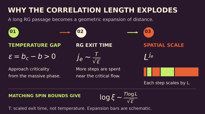
Set and rescale logarithmic distance by . Dividing the two coordinates by gives limiting variables and satisfying and . Their explicit solution is:
Here denotes a scaled exit time, not physical temperature. The invariant fixes the solution. The outgoing pole occurs at , so the discrete exit index satisfies .
Each RG step multiplies spatial distance by . Therefore the exit length grows on the scale . This is where the BKT essential singularity acquires its exponential form: a reciprocal-square-root number of steps becomes a geometric spatial expansion.
The proof stops at a sufficiently small fixed outgoing activity. It does not run the map into an uncontrolled strong-coupling regime. Illustratively, quartering the parameter distance doubles the leading logarithmic length, approximately squaring the leading exponential scale. That is a scaling illustration, not a numerical prediction for a material.
The cotangent and cosecant formulas also explain the square root quantitatively. Near zero, their expansions match the critical trajectory plus its temperature displacement. This fixes the conserved quantity through the response coefficient . The passage time is therefore tied to the microscopic temperature derivative, rather than fitted after observing the divergence.
10. Why The Dual-Height Fluctuation Profile Jumps From Eight Pi To Zero
The exit length still needs a physical interpretation. The paper studies , the variance of an affine height test comparing opposite face averages on a free square. On moving scales , subsequences yield a nonincreasing limiting profile .
Cutting comparisons, uniform moment bounds and Gaussian height limits constrain this profile. A relative-growth estimate excludes intermediate positive values. Torus variance diagnostics then locate the change at the same exit time:
The coefficient belongs to the paper’s height spacing and Laplacian normalization. Zero means the selected macroscopic fluctuation coefficient vanishes, not that every microscopic height becomes identically zero. The paper asserts no limiting value at the jump itself.
This is a profile across jointly diverging scales and approaching temperatures. It should not be confused with an ordinary thermodynamic order-parameter discontinuity. Keeping the observable straight matters just as much in the 2D area-law problem, where entanglement entropy and ordinary correlations carry different information.
Excluding intermediate coefficients prevents a long crossover plateau from shifting the leading length scale. Establishing Gaussian limits in pinned geometries is equally necessary: the later spin argument uses an exterior height fixed to zero, whereas a free height field retains an arbitrary common translation. Those boundary conventions cannot be interchanged without proof.
11. Connecting Renormalization Flow To Spin Correlations: The Final Proof
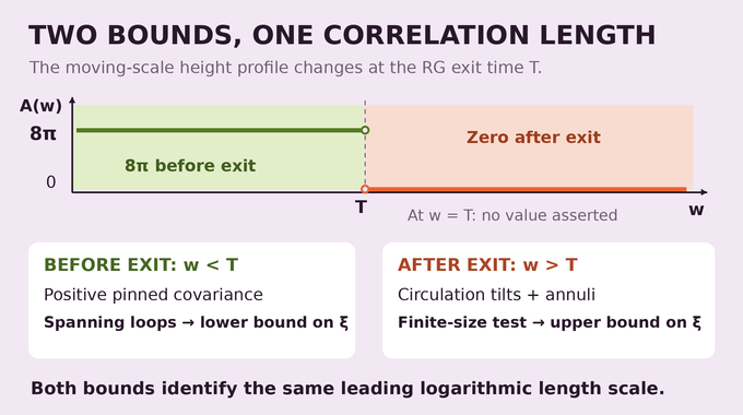
Below the exit time, pinned-height limits have positive covariance between separated interior regions. In the exact loop representation, such covariance requires loops spanning macroscopic distances. If the spin correlation length were exponentially smaller, correlation inequalities would suppress those loops and force the covariance to vanish. This gives the lower bound on length.
Above the exit time, affine height variances vanish uniformly over suitable logarithmic-scale intervals. Fixed circulation tilts then have arbitrarily small fluctuation cost. Stacking annuli around a spin insertion produces correlations smaller than any prescribed inverse power at those scales.
The Lieb–Rivasseau finite-size criterion upgrades that finite-scale smallness to a positive lower bound on mass, hence an upper bound on length. As in the Haldane gap problem, estimates must survive increasing system size rather than merely look convincing on finite samples.
| Scale Window | Height Evidence | Spin Consequence |
|---|---|---|
| Before Exit | Positive separated pinned covariance. | Correlation length cannot be exponentially smaller. |
| After Exit | Vanishing affine fluctuations and inexpensive circulation tilts. | Finite-size criterion bounds correlation length from above. |
Both bounds converge to the same logarithmic scale. A subsequence contradiction removes extraction and establishes the full limit, respecting the prescribed boundary and separation limits.
12. What The BKT Transition Proof Resolves And What Remains Unevaluated
The amplitude is . Although intermediate parameters depend on the block construction, the final amplitude is determined by the original model. Neither its closed-form value nor a numerical critical temperature is calculated.
The critical-exponent companion and the logarithmic-correction companion supply the critical exponent , logarithmic correction , critical height limits and analytic activity map. These are dependencies, not additional main theorems proved from scratch here. The result concerns the specified square-lattice cosine interaction, without automatically covering every XY-type model or experimental system.
OpenAI’s release announcement attributes the collection to an internal frontier model. That provenance does not establish peer review or complete machine verification of this argument. This remains an October 2026 research preprint, and this review does not certify a full Lean formalization. Our guide to AI mathematical proofs explains why those evidence categories matter.
For researchers and simulation developers, the useful target is a controlled asymptotic law and a route connecting microscopic weights to observable correlations. The paper reports no software speedup or material-device benchmark. Applying the theorem to finite simulation data would still require estimating criticality and controlling finite-size effects, neither of which disappears because the asymptotic law is known. The BKT transition story advances through those mathematical bridges. Follow Binary Verse AI for research explainers that examine the theorem, assumptions and proof mechanism together.
What did OpenAI prove about the BKT transition?
OpenAI’s October 2026 preprint proves the essential singularity of the correlation length for the nearest-neighbor cosine XY model on the square lattice. It establishes that approaches a finite, strictly positive constant as inverse temperature approaches criticality from the massive phase.
Was the BKT transition already mathematically proved before OpenAI’s work?
Yes. Earlier rigorous results established the existence and important properties of the BKT transition. The advance here is the precise leading logarithmic correlation-length asymptotic for the original cosine XY model, including a single positive limiting amplitude.
Why does the BKT correlation length diverge exponentially instead of following a power law?
The critical renormalization flow has an exit time proportional to . Successive RG steps increase spatial scales geometrically, producing an exponentially large length. The proof then establishes that this scale matches the actual spin correlation length at leading logarithmic order.
How does the proof connect renormalization flow to physical spin correlations?
It establishes a sharp change in the dual-height fluctuation profile. Positive pinned-height covariance yields a lower bound on correlation length. Circulation estimates and a finite-size criterion yield the upper bound. Together they identify the RG exit scale with the correlation-length scale at leading logarithmic order.
Does the proof rely on approximating the XY model as a Gaussian field?
It retains the original cosine interaction through an exact current and Bessel-height representation. Gaussian comparison inequalities and rigorous Gaussian height limits are used within the argument. The microscopic XY model is not replaced by a Gaussian approximation.
Does OpenAI’s proof calculate the exact BKT critical temperature or correlation-length amplitude?
No. It proves that the limiting amplitude exists and is strictly positive and finite. The proof expresses it through renormalization parameters but does not evaluate it in closed form or determine a numerical critical temperature.