
Prescribe every displacement pattern you can on the surface of a solid and record the force per unit area needed to hold each one. Could two bodies with the same shape but different interior stiffness give exactly the same responses? OpenAI’s preprint on isotropic elasticity proves they cannot under its smooth, three-dimensional, static model. The complete boundary response determines two spatially varying stiffness parameters, the Lamé moduli. The proof uses the boundary data to transfer exact elastic solutions between candidate materials and compare their behavior across a complex family of directions.
Table of Contents
1. Isotropic Elasticity: What Exactly Did OpenAI Prove?
Theorem 1.1 of the original manuscript fixes a bounded, connected domain in three-dimensional Euclidean space with smooth boundary. It compares two pairs of real Lamé parameters that are smooth up to the boundary and satisfy and on the closure. If both pairs produce the same static Dirichlet-to-Neumann map, their respective and agree at every point of the body.
| Feature | What the Theorem Uses or Proves |
|---|---|
| Setting | Static, linear isotropic elasticity on a known bounded, connected domain with smooth boundary in three dimensions. |
| Unknowns | Two real, spatially varying Lamé moduli, and , smooth up to the boundary. |
| Positivity | and on the closure. |
| Data | The full displacement-to-traction map at zero frequency. |
| Conclusion | Identical maps force identical moduli throughout the domain in fixed Euclidean coordinates. |
The positivity conditions give positive elastic energy for nonzero strains and support the well-posed forward problem. The theorem permits arbitrary smooth spatial variation within that class. In particular, the two candidate materials enter the comparison without a prescribed common collar near the boundary. The proof deduces boundary agreement from the measurements themselves.
2. The Original Inverse Problem: Can a Surface Reveal the Interior?
In the forward problem, the material is known. Prescribe the surface displacement, solve for the equilibrium displacement inside, then compute the traction, the local force per unit area on the surface. The inverse elasticity problem starts from that response operator and asks which material produced it. Isotropy means that the linear response at each point has no preferred direction. The stiffness may still vary from point to point. The model describes small, reversible elastic deformations. Plastic deformation leaves a permanent change after unloading and falls outside this constitutive law.
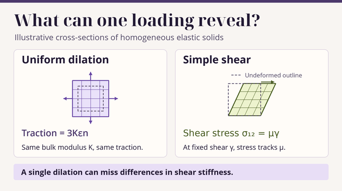
Even a full traction field from one loading can be blind to part of the material. Take a homogeneous body and prescribe a uniform infinitesimal dilation with displacement . In equilibrium its strain is and its traction is , where is the bulk modulus and the outward unit normal. Two constant pairs with the same and different shear moduli give exactly the same traction for this loading. Another displacement pattern, such as simple shear, can distinguish them. For , where is the imposed shear, the volume strain is zero and the off-diagonal stress depends directly on the shear modulus. These affine fields solve equilibrium for constant coefficients because the corresponding stresses are constant. Spatially varying coefficients generally require solving the interior equation even for a simple boundary pattern.
3. Lamé Parameters, Stress, Strain, and Boundary Measurements
The symmetric displacement gradient gives the infinitesimal strain . Its trace, , measures first-order volume change. Isotropy makes the stress a linear combination of that trace times the identity and the strain itself. With no body force, equilibrium requires zero stress divergence.
Writing strain as its trace-free part plus uniform dilation shows why governs shear and governs volume change. For smooth boundary displacement , let be its equilibrium solution. The displacement-to-traction map is . In the paper the operator acts on the Sobolev trace space and takes values in its dual , where traction is defined by the elastic energy pairing. Equality means the same operator for every admissible vector-valued boundary displacement on the entire surface.
4. Why Three-Dimensional Uniqueness Remained Difficult
The scalar conductivity Calderón problem also asks what a boundary operator reveals about an interior coefficient. Elasticity couples two moduli through three displacement components. Nakamura and Uhlmann’s original global result was corrected by their 2003 erratum. A prescribed planar matrix transport initial-value problem could fail to have a solution, and the corrected substitution led to a pseudodifferential equation where the original proof had asserted a partial differential equation. The corrected uniqueness theorem required both shear-modulus gradients to be sufficiently small in a specified differentiability norm.
Earlier three-dimensional results also used analyticity or particular structures, such as axisymmetric or separable shear moduli in specified geometries. Imanuvilov and Yamamoto had already proved the smooth two-dimensional theorem under its own positivity conditions. The new three-dimensional argument has to extract useful interior equations from physical displacement data. The noninjective auxiliary-field map in earlier reductions is one reason this step needs its own proof.
5. The First Breakthrough: Transferring Physical Solutions Across the Boundary
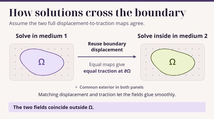
Equality of the two boundary maps fixes the boundary jets of the moduli, which record their values and derivatives of all orders on the surface. Using Tan and Liu’s boundary determination theorem, the paper extends both pairs smoothly to all of space, with common coefficients on the complement and a common constant pair far away. Matching jets make the extension smooth even across boundaries of cavities. An extension of the first pair can be blended with a constant using a cutoff because the admissible set defined by the two strict inequalities is convex.
Start with an exact solution of the first elasticity equation on a ball containing the body. Solve the second equation inside the body using the first solution’s boundary displacement. Equal displacement lets the fields be glued, and equal traction cancels the interface terms in the weak equation. Elliptic regularity then makes the glued solution smooth. The two fields agree throughout the exterior, as do their divergences. Their difference is supported in the closure of the body, so the later weighted estimate can be applied on a larger ball without imposing boundary values on that ball.
6. Reducing Elasticity to a Four-Component Laplace-Type System
Write , and . The paper temporarily treats the scalar as independent of the three-component displacement . The vector expression expands the physical elasticity equation with in place of the displacement divergence. The scalar expression is arranged so that their mismatch is a differential operator applied to the divergence defect.
Here . For an exact physical solution with , both and vanish. Subtracting from cancels its second derivatives of . Dividing the vector equation by and the resulting scalar equation by gives a system with principal part , the same scalar Laplacian on all four components. Thus the two media’s normalized operators differ only in terms of first order or lower. The comparison uses physical pairs throughout, which keeps the scalar component tied to the actual displacement.
7. Carleman Estimates and Complex Geometric Optics Solutions
The proof uses complex geometric optics solutions with exponential factor , where is large and is a nonzero complex vector with . The dot product is complex bilinear. Applying the Laplacian to the exponential would normally produce a term quadratic in . The null condition cancels it, so the leading equations for the amplitudes involve the first-order direction derivative . The real and imaginary parts of have equal length and are orthogonal. They span the plane where acts as a multiple of the Cauchy–Riemann operator, with the transverse coordinate held fixed.
The Carleman estimate bounds a compactly supported pair after its exponential has been factored out. Its gain of order offsets a first-order forcing of order in the comparison step. The construction also uses a high-order amplitude expansion that respects the divergence constraint order by order. It corrects the residual with the physical elasticity operator. Taking the divergence of that correction can cost a factor of , so the expansion makes the initial error small enough to control both the displacement and the actual divergence.
8. Building Three Independent Transport Solutions
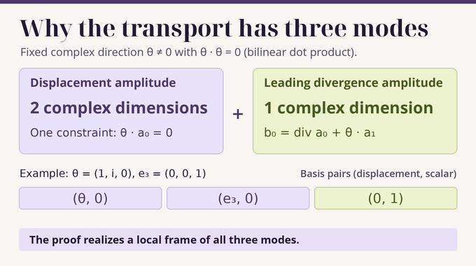
Let be the leading displacement amplitude and its first correction, multiplied by . The conjugated divergence starts with , which must vanish to keep the divergence bounded. The leading scalar amplitude then includes both and . This second contribution is why the transport can carry an independent scalar even though the exact pair always contains a physical divergence.
The orthogonality condition cuts the displacement amplitudes down to a complex two-dimensional plane. Together with the scalar, the transport has three dimensions. For example, with , both and lie in and form a basis for it. Adding the pure scalar direction gives a basis of the fiber. The proof builds a smooth invertible transport frame on planar disks for a local interval of transverse coordinates. It then realizes each column as the leading pair of an exact physical solution. These columns let the comparison test every polarization the transport can carry.
9. Matching the Transports Through Holomorphic Comparison
An invertible change of amplitudes gives and . The normalized transport has a common upper equation . Write for the full transport matrix in medium . Transfer the first medium’s three exact solutions into the second. Because the augmented operators have the same principal part, the supported Carleman estimate bounds the transferred amplitudes in . Weak limits satisfy the second transport in distributions and keep the exterior agreement. In the divergence relation for the transferred pair, division by leaves as the only term that can survive in the distributional limit. Thus the limiting displacement amplitude still lies in the constrained plane. This step places both sets of columns in the same fiber before the two transport systems are compared.
Put the normalized columns in and . Only the original frame needs to be invertible to form . The comparison satisfies
Here is a fixed ball containing the body. Supported planar uniqueness lets the local comparisons agree wherever they overlap. Estimates on fixed supported Sobolev spaces give smooth dependence on position and direction. The manuscript credits earlier transport comparison for connection Laplacians. A related one-patch Calderón theorem asks what partial boundary data determine about a metric and connection.
Nonzero multiples of describe the same point of the projective null conic . In a holomorphic conic chart, differentiating the comparison equation in the conjugate direction coordinate at fixed spatial position gives a supported homogeneous equation. Uniqueness makes that derivative zero. Thus is holomorphic on the conic for every .
10. The Geometric Argument That Forces the Comparison to Be Identity
The displacement planes form a holomorphic bundle over the conic, which is a projective line. Any global holomorphic section of has constant ambient coordinates by compactness. Such a constant vector is orthogonal to all null directions, which span , so it vanishes. The paper also shows that the quotient of by the null line bundle with fiber is a trivial line bundle. Indeed, on the projective line and , where is the tautological line bundle. In projective coordinates , the null line sits inside the two copies of along the column . The row kills precisely that line and is surjective at every point. This gives the trivial quotient explicitly and explains why the geometry can rule out a block of the comparison.
The block of mapping the scalar into the displacement plane is therefore zero. The scalar-to-scalar block is independent of direction by compactness. Let be the displacement block and the displacement-to-scalar block. The common upper transport equation gives . Therefore factors through the trivial quotient . Such a map into would give a global holomorphic section, so it vanishes. The remaining upper block equation is
The right side has rank at most one, while a nonzero multiple of the identity on has rank two. Hence and . The null directions span the ambient space, so is also constant in space. The exterior value forces , giving and equality of the two transports.
11. Recovering Both Lamé Moduli and the Limits of the Result
The scalar diagonal of the normalized transport is . Its equality in all null directions forces the two logarithms to differ by a constant. Exterior agreement sets that constant to zero. Thus everywhere. One ratio leaves the overall shear scale to be determined.
The other lower block acts on . Its equality allows the ambient covectors to differ by a multiple of , since that line annihilates under the bilinear dot product. The difference is linear in . Its proportionality factor is holomorphic on the compact conic and therefore independent of direction. Because null vectors span, the ambient matrix giving this difference is a scalar multiple of the identity. Subtracting the paper’s coefficient formulas, with , now yields
The are smooth functions of the two candidate media. The scalar accounts for the identity ambiguity and is the Kronecker delta. Differentiating a diagonal equation and commuting third derivatives with an off-diagonal equation expresses each derivative of in terms of and . For a derivative in direction , choose an index and use . The off-diagonal equation contains no , which lets this identity isolate . The Hessian equation already expresses the derivatives of in those terms. Along a path, this closed homogeneous system becomes a linear ordinary differential equation. Both quantities vanish in the common exterior, so ordinary uniqueness propagates their vanishing everywhere. Therefore . With the shear moduli equal, the shared ratio then fixes .
OpenAI’s release announcement describes the research program. The family 372 scope note identifies the Lean result as global uniqueness for the full static map under the stated smoothness and positivity hypotheses. The accompanying Lean proof source concludes equality of both coefficient functions from equality of the boundary maps. Reconstruction would require a procedure for computing the moduli from data. Stability would require a bound on how measurement errors affect the recovered moduli. Limited surface access, noise and wave-based imaging call for additional analysis.
The result gives isotropic elasticity an identifiability theorem for both smooth moduli from full static data. Its decisive step is turning boundary agreement into a transport comparison stringent enough to leave only the identity. Follow Binary Verse AI for more research explainers that trace what a theorem establishes and how its proof gets there.
Can boundary measurements uniquely determine a material’s internal elastic properties?
Yes. OpenAI proves that the complete static displacement-to-traction map uniquely determines both smooth Lamé moduli throughout a three-dimensional isotropic elastic body satisfying the theorem’s assumptions.
What are the Lamé parameters in isotropic elasticity?
The Lamé moduli λ and μ describe an isotropic material’s linear elastic response. The shear modulus is μ, while the bulk modulus is K = λ + 2μ/3. Both may vary spatially in the theorem.
Why did earlier proofs of three-dimensional elasticity uniqueness need additional assumptions?
Earlier results used restrictions such as small shear-modulus gradients, analyticity or particular coefficient structures. The corrected Nakamura–Uhlmann theorem requires both shear-modulus gradients to be sufficiently small.
Does OpenAI’s uniqueness proof also apply to two-dimensional elasticity?
The manuscript proves the three-dimensional case. Imanuvilov and Yamamoto had already established global uniqueness for smooth two-dimensional isotropic elasticity under the positivity conditions μ > 0 and λ + μ > 0.
Can a single surface indentation determine both Lamé moduli?
A single force–displacement measurement can leave multiple parameter combinations indistinguishable. The theorem assumes the complete displacement-to-traction map, which describes the response to every admissible boundary displacement.
Does the OpenAI proof provide a reconstruction algorithm for internal stiffness?
The proof establishes that identical complete boundary responses force both Lamé moduli to agree everywhere. A numerical procedure for computing them and a stability estimate for noisy measurements are separate problems.
Does this proof solve practical seismic imaging or medical elastography?
It proves uniqueness for ideal static isotropic elasticity. Practical seismic imaging and wave-based elastography need additional analysis for wave dynamics, limited measurement access and noise.