
If every legal expression has a terminating reduction, must every reduction strategy terminate? For pure type systems, OpenAI’s September 2026 manuscript answers yes under a system-wide hypothesis. If every legal expression in every valid context can reach a β-normal form, then no infinite β-reduction sequence can start from any of them. Weak vs strong normalization comes down to which reduction paths the claim quantifies over. The proof makes that jump by tracking the sorts a type can inhabit and showing that the resulting dependencies cannot support a particular typed diagonal construction.
Table of Contents
1. Weak vs Strong Normalization: Why One Terminating Path Is Not Enough
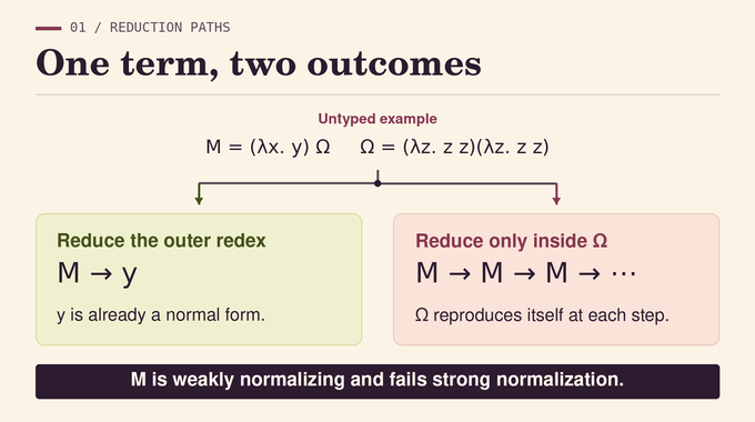
A β-redex is an application whose function is a lambda abstraction. A normal form contains no redex anywhere. Weak normalization asks whether you can reach such a form by choosing redexes in some order. Strong normalization asks whether an infinite sequence is possible under any choice.
| Concept | Meaning |
|---|---|
| Weak normalization | At least one β-reduction path reaches a normal form. |
| Strong normalization | No infinite β-reduction path starts from the expression. |
| Theorem 1 | Weak normalization implies strong normalization for the whole pure type system. |
| Scope | Legal expressions in every valid context, including open terms, types, and reductions inside annotations. |
| Specification | Sort axioms and product rules may be nonfunctional. |
For a worked example of normalization in lambda calculus, take to be . Contracting its outer application gives back . Now let , where is a variable distinct from .
The first step discards the argument. The second contracts a redex inside the argument and returns to exactly the same expression, so it can be repeated forever. Thus is weakly normalizing and fails strong normalization. The example concerns a raw expression. The theorem assumes weak normalization for all legal expressions in the system.
2. The Barendregt–Geuvers–Klop Conjecture: What Was the Original Problem?
Geuvers’s 1993 thesis formulated the conjecture for β and βη reduction. Theorem 1 of OpenAI’s normalization manuscript establishes the β case for arbitrary pure type specifications. A typing judgment says that the subject has expected type under the declarations in . The context is valid when each declaration’s type is assigned a sort using the preceding declarations. An expression is legal if it occurs as either the subject or the expected type of a derivable judgment. Declaration types are covered because context validity requires their own sorting judgments.
The universal quantifier appears twice. Every legal expression in every valid context must be weakly β-normalizing, and the conclusion then gives strong β-normalization for every expression in that same range. The proof needs the full hypothesis because the auxiliary expressions it builds must also have normal forms.
3. Pure Type Systems, Dependent Types, and Full β-Reduction
A pure type specification gives a set of sorts , a relation telling which sorts classify other sorts, and a relation listing permitted dependent product formations. A rule says that a domain of sort and a codomain of sort can form a product of sort . The codomain is checked under an added declaration for the bound variable, so can describe a function whose result type depends on its input. Applying a function of that type to yields the type .
The β rule substitutes the argument for the free occurrences of the binder in the body, renaming bound variables when necessary to avoid capture. A step is also allowed under a binder and in either part of a product or application. For example, a lambda with a variable as its body still admits a step if its domain annotation contains a redex. The context supplies types for free variables and is external to the expression being reduced.
The specification need not assign a unique target sort to a sort axiom or to a pair of input sorts in a product rule. The same syntax can therefore have several legitimate sort derivations, which the proof must handle together.
4. Why Earlier Normalization Proofs Could Not Reach Every Pure Type System
Sørensen used a continuation-passing translation to turn divergence of an original term into failure of weak normalization for a translated term. The translation must preserve typability. To type the extra functions introduced by passing continuations, its construction relies on available products and on structural assumptions. The manuscript describes Sørensen’s result for generalized nondependent, clean, negatable systems and the development of the nondependent approach by Barthe, Hatcliff, and Sørensen.
Mull relaxed cleanliness and negatability conditions in the nondependent tiered setting. There the sorts form a finite axiom chain, and each product inherits the sort of its codomain. An arbitrary specification can lack the product rules a translation needs and can allow dependent codomains and circular sort dependencies. OpenAI’s proof works with the rules already present. It uses their structure both to build the normalization argument and, when a certain pattern occurs, to type the expression that defeats the hypothesis.
5. The First Proof Step: Finite Specifications and Unique Normal Forms
Suppose a legal expression admits an infinite reduction. A literal sort is already normal, and every other legal expression is typable. Its typing derivation uses finitely many sorts, axioms, and rules. The proof also retains the sorts in the finite conversion chains used by that derivation. Full β-reduction creates no new sort symbols. The infinite path therefore survives in the restricted specification, as do the finite normalizing paths supplied by the hypothesis for expressions legal there.
Confluence says that two reducts of a common expression can be joined. Combined with weak normalization, it gives each legal expression a unique normal form up to renaming bound variables. Write for that form. Subject reduction preserves the exact expected type when the subject takes a β-step. In particular, normalizing a sorted type preserves its sort.
The paper then builds a saturated context into which every finite valid context embeds after renaming. Each actual judgment still lives over a finite prefix. Any finite collection of judgments can share a long enough prefix, and fresh variables of already sorted types are always available. This lets the proof test open terms together without dropping their typing assumptions.
6. Sort Profiles: How OpenAI Handles Types with Multiple Sorts
The profile of an expected type records every sort derivable for its normal form in the context .
For a literal sort, the profile consists of its axiom targets and can be empty. A sorted normal neutral expression, meaning a variable with zero or more arguments, has a singleton profile. For a normal product, take all outputs of formation rules whose first sort belongs to the domain profile and whose second belongs to the codomain profile in the extended context. For example, a rule set allowing the same input pair to produce two distinct sorts puts both into the product’s profile.
A nonempty profile is feasible if it occurs in a valid context. The finite specification yields finitely many feasible profiles. The proof generates them from nonempty axiom profiles and suitable singletons, closing under nonempty product outputs. Typed substitution preserves the old sorts but can expose additional ones. A neutral type can become a product after substituting for its head and normalizing. Keeping only one sort would lose the information needed to track that change, while requiring profile equality would rule out legitimate substitutions.
7. Reducibility Candidates: Testing Every Strongly Normalizing Application
Two expressions can separately be strongly normalizing while their application diverges. In the untyped example, each copy of is already normal, but their application is . The strong normalization proof has to show why the typing rules exclude this kind of interaction.
For a normal actual type , the paper considers finite stacks of strongly normalizing arguments. A stack starts with an argument of the function’s domain type. The next argument is checked against the type obtained by substituting the first argument into the codomain and normalizing, and so on. An empty stack tests the function itself. The set consists of terms at that remain strongly normalizing under every such test. The larger set requires only typed strong normalization of the term by itself.
In the Tait–Girard tradition, a candidate lies between those sets and is closed under a controlled head expansion. If the contracted application belongs to the candidate, it can be expanded back when its annotation, body, argument, and remaining stack entries are all strongly normalizing. For dependent products, the interpretation must give a candidate equal to its product test. The introduction direction admits lambdas, while the elimination direction tests applications. A separate specialization law aligns the tested result with the candidate of the substituted codomain.
8. Signed Dependency Graphs: The Structure Behind the Proof
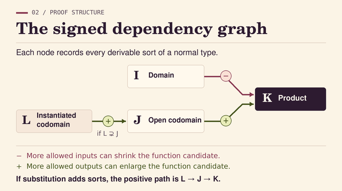
Each feasible profile becomes a vertex. A product with domain profile , open codomain profile , and product profile gives an edge from each child to the product. The domain edge is negative because enlarging the set of tested arguments can only shrink the set of functions that pass, with codomain tests fixed. The codomain edge is positive because allowing more outcomes can only enlarge the passing set. A strict profile enlargement gives another positive edge, from the larger set of sorts to the smaller one.
The diagram follows one product and its instantiated result. Substitution can enlarge the codomain profile from to , so there is a positive route from to through . This keeps the instantiated type within the dependency order the proof needs.
A strongly connected component groups vertices that can reach one another in both directions. The proof processes predecessor components first. A closed walk with an odd number of negative edges reverses the comparison direction on return to its starting point. That conflict is what the first construction must avoid.
9. From Easy Components to the Hard Case: Fixed Points and Observation Spaces
When a component has no odd closed walk, its vertices can be assigned consistent signs. Reversing the inclusion order at the negatively signed vertices makes the candidate operator monotone on a complete lattice. Tarski’s fixed-point theorem supplies the simultaneous interpretation. A second construction works when no product has its domain, codomain, and result profiles all in the component. At most one child is then internal for a product in that component, and the construction uses signed comparisons to track changes under substitution.
The remaining components need observation spaces because a type that appears neutral before substitution may reveal a product afterward. An observation table is queried by a finite stack of typed normal arguments and auxiliary values where needed. It can record a base candidate assignment and continue at the normalized result type. The argument payload and the result may themselves require tables, so their spaces can depend on one another.
For some profiles, the paper builds tables along finite paths or by a decreasing count of selected type nodes. For the remaining spaces it alternates stages of tables, with unrestricted tables on one side and tables that depend on a bounded stage of opposite payloads on the other. The stage bound is uniform across observations of a fixed typed expression, even when argument choices and stack lengths vary without bound. It controls what the table can inspect, rather than the number of β-steps. Substitution and reduction transport then connect the candidate tested before instantiation to the candidate read from the normalized result type.
10. Hurkens’s Paradox and the Guarded Diagonal Argument
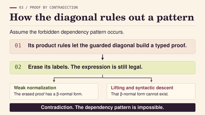
The decreasing count can fail if substituting an argument turns a neutral leaf into a product whose new nodes would be counted. Condition (7) excludes the graph pattern that permits this failure. It combines an internal negative dependency in a plain active secondary component, a product with codomain and result there, and a positive path from the axiom profile of a sort whose singleton profile is in that component to the product’s domain profile. A plain profile reaches the designated test-domain profiles along both even and odd paths.
The exclusion uses a typed adaptation of Hurkens’s well-foundedness paradox. The available product rules yield a formula calculus with proof and data labels, including quantifiers over specific supported data types. Two data channels supply predicates and observations. Their access construction preserves an open parameter exactly and rounds another argument to a representative. The relational coding tracks when queries are admissible and when predicates respect observational equivalence. A biconditional between formula observations alone cannot justify replacing data inside an arbitrary function.
The diagonal defines a predicate by negating a test against extensional predicates. The guards are the validity and extensionality conditions that allow the necessary comparisons and self-reference to be typed. The construction produces a proof-mode term at a designated terminal formula in a valid open context. A separate descent argument rules out a proof-mode inhabitant there with normal erasure. Erasing the labels keeps all annotations, and every ordinary typed β-step lifts back to a labelled step preserving proof mode. Weak normalization of the erased term would thus give the very normal erasure the descent excludes.
11. Completing OpenAI’s Proof: Why Every β-Reduction Sequence Terminates
Once the forbidden configuration is excluded, every component has the required interpretation. Processing the graph proves at every actual type. Now choose a smallest typable expression that fails strong normalization. Its children are strongly normalizing, including those inside binders and annotations. Variables and sorts are normal, and a binder with strongly normalizing children cannot diverge. The remaining possibility is an application. Its function passes the one-argument test because equals , contradicting the choice of expression.
The manuscript supplies the mathematical argument. OpenAI’s Lean scope note for family 245 reports a formalization with the same β-only scope, including arbitrary sorts, nonfunctional rules, and annotations. The public Lean comparator specifies the target theorem with a sorry placeholder. Independent review can examine how the encoded statement corresponds to the manuscript. The project was announced in OpenAI’s October 2026 mathematics release.
The weak vs strong normalization theorem gives type theorists a concrete proof route. Establish a normal form for every legal expression in every valid context, and termination follows for every β-reduction path. The manuscript treats full β-reduction and leaves the βη implication outside its scope. It gives no practical bound on reduction time or cost. Explore more Binary Verse AI coverage of machine-checked mathematics in our Fermat’s Last Theorem Lean explainer, percolation theory formalization, and analysis of the Navier–Stokes Lean proof’s scope.
What is the difference between weak and strong normalization?
Weak normalization means an expression has at least one β-reduction sequence that reaches a normal form. Strong normalization means no infinite β-reduction sequence starts from that expression. Strong normalization implies weak normalization. An individual expression can have a normal form and still admit an infinite sequence.
Can a weakly normalizing expression still have an infinite reduction sequence?
Yes. In the article’s untyped example, the outer function discards its argument and returns a variable immediately. The argument is a self-application that reproduces itself in one step. Reducing only that argument produces an infinite sequence from the same starting expression.
Does weak normalization imply strong normalization in pure type systems?
Yes, under the paper’s system-wide hypothesis. OpenAI proves that if every legal expression in every valid context of a pure type system is weakly β-normalizing, then every such expression is strongly β-normalizing.
Why was the Barendregt–Geuvers–Klop conjecture difficult to prove?
Earlier arguments needed structural conditions governing type dependencies, sort hierarchies, or which products could be formed. An arbitrary pure type system can have circular dependencies and several outputs for the same input sorts. Those systems require a more general argument.
Why does OpenAI’s proof use Hurkens’s paradox?
A typed adaptation excludes a specific pattern in the dependency graph. The pattern would let the authors construct a legal open expression with no β-normal form, contradicting system-wide weak normalization.
Does the proof cover dependent types, open contexts, and η-reduction?
It covers dependent products, valid open contexts, and β-reduction inside type annotations for arbitrary pure type systems. Its scope is β-reduction. The manuscript leaves the corresponding βη implication outside the theorem.
Has OpenAI’s normalization proof been formalized in Lean?
OpenAI’s family 245 scope note reports a Lean formalization of the β result. The public comparator specifies the target statement and marks its proof with a sorry placeholder. The comparator serves as a checking interface for the formalization. Independent mathematical review is a separate step.