
A density can come from a real interacting Coulomb ground state yet have no exact Kohn–Sham stand-in within a familiar class of local potentials. OpenAI’s manuscript constructs precisely that situation with three electrons and two nuclei. Its Kohn–Sham representability result survives arbitrary mixtures of noninteracting ground states. The obstruction lies in a tiny density tail on a symmetry plane, where interaction creates something an admissible common orbital potential cannot reproduce. This is a mathematical existence result, with no accompanying benchmark of everyday DFT errors.
Table of Contents
01. What OpenAI’s Proof Establishes About Kohn–Sham Representability
Theorem 1.1 of the original Coulomb counterexample paper supplies a finite molecule with equal positive integer nuclear charges. Its spin-summed ground-state density cannot be reproduced by any three-electron noninteracting ground-state ensemble in a single real, spin-independent local potential belonging to . This sum space permits an integrable singular part plus a bounded part, including ordinary nuclear Coulomb potentials.
| Question | Verified Scope |
|---|---|
| System | Three interacting electrons and two equal integer-charge nuclei. |
| Density | Spin-summed, with . |
| Excluded representations | All noninteracting ground-state ensembles in . |
| Not established | Failure of DFT generally, or exclusion of every generalized potential. |
The manuscript presents an analytic proof. It does not report machine-checked formalization of this theorem or practical calculation speeds. Reading an “OpenAI Kohn–Sham proof” as a statement about a particular mathematical model keeps its significance precise.
The potential class is broad enough to allow singular nuclear attractions and bounded behavior at infinity. Excluding this entire class is stronger than showing that a smooth or symmetry-restricted trial potential fails. Conversely, the function-space restriction remains part of the theorem and must accompany any summary of the result.
02. Why the Kohn–Sham DFT Mapping Was Never Guaranteed
In Kohn–Sham density functional theory, interacting electrons are replaced by noninteracting electrons chosen to reproduce their density. Their orbitals feel one common local Kohn–Sham potential. The original Kohn–Sham formulation makes this auxiliary description central to the method.
Interacting v-representability means a density is realized by an interacting ground state in an external potential. Noninteracting v-representability asks whether a noninteracting ground state can realize it. The Hohenberg–Kohn density–potential relationship does not turn the first existence question into an affirmative answer to the second.
Ensemble v-representability broadens the search by mixing degenerate ground states. For example, averaging two equal-energy determinants can produce a density absent from either determinant alone. Proving one selected determinant impossible therefore leaves an important escape route. This paper closes that route for its constructed density, within the stated class.
There is also a distinction between constructing some antisymmetric state with a prescribed density and making that state an energy minimizer for a local potential. Constrained search solves the former optimization problem without guaranteeing the latter potential. The counterexample exploits precisely this gap between a density constraint and a representing Hamiltonian.
03. The Earlier Mathematical Obstacle: Why Previous Counterexamples Were Not Enough
Earlier examples prescribed densities whose inverse potentials leave the admissible space. Such constructions distinguish density regularity from potential regularity, but do not automatically exhibit a finite Coulomb molecule producing the problematic density.
The manuscript also discusses atomic density-inversion evidence. Numerical inversion can reveal serious difficulties, yet an unsuccessful reconstruction does not exclude every potential, degeneracy, or ensemble. A theorem needs stronger control than a solver’s failure.
The closest mechanistic predecessor is research on density tails near a highest-occupied-orbital nodal plane. It identified how ionic-channel coupling can preserve a slow exponential decay rate on the plane while adding polynomial suppression. The new construction combines that mechanism with Coulomb estimates, an all-ensemble certificate, and an exclusion covering the entire sum space.
The historical advance is therefore not the first observation of a representability difficulty. It is the combination of a genuine finite Coulomb ground state with a proof robust to every admissible ensemble. Earlier asymptotic reasoning motivates the construction, while the new spectral and variational arguments establish the universal exclusion.
04. The Three-Electron Coulomb Molecule at the Heart of the Proof
Place two nuclei of charge at , where . Three electrons experience nuclear attraction and mutual Coulomb repulsion, with kinetic term in atomic units. The nuclear positions are fixed parameters of this electronic Hamiltonian.
Theorem 1.1 supplies a normalizable absolute ground state in the sector . “Absolute” matters: the construction is not merely a lowest state inside an artificially restricted excited sector. Its density sums over spin and integrates out the other two electron positions.
The excluded auxiliary system must reproduce that density almost everywhere, using three noninteracting fermions and the same scalar potential for both spins. The distinction from electronic-structure computational hardness is useful: hardness concerns the resources needed to solve a problem, whereas this theorem concerns whether a specified auxiliary representation exists.
05. The Scaling Argument and the Two Lowest Electron Orbitals
Set . Dividing the transformed Hamiltonian by gives unit nuclear charges at and repulsion strength :
The two lowest normalized spatial orbitals are a positive even orbital and an odd orbital , positive above the median plane. Their energy splitting is positive and becomes small as scaled separation grows. Higher levels remain spectrally isolated.
At zero coupling, occupy , , and . The density is . Small positive coupling continues this state while retaining the required bound-ground-state properties. Scaling back gives and preserves the representability obstruction.
The order of limits matters. The proof first fixes a sufficiently large scaled separation, then chooses a sufficiently small positive coupling. It does not replace the final molecule by infinitely separated nuclei or switch off electron repulsion. The selected system remains finite, and its nonzero interaction is indispensable to the planar tail.
06. How the Nodal Plane Creates the Decisive Density Tail
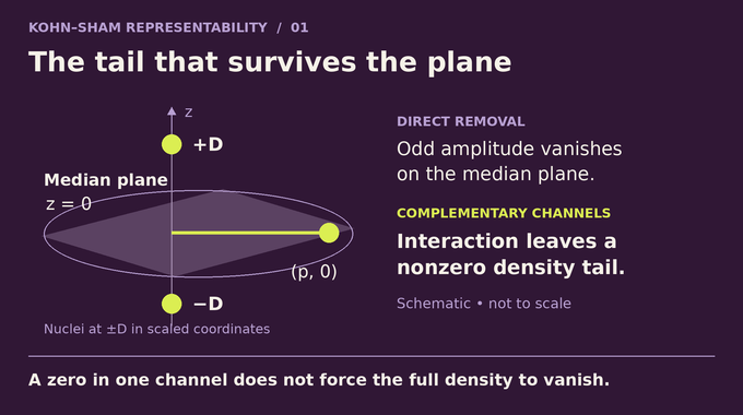
Think of removing one electron and resolving the remaining pair into ionic channels. Projection onto the ionic ground state gives the direct removal amplitude. Its odd angular factor vanishes on the median plane. Complementary ionic channels carry the interaction-induced correction.
Write , where and are scaled ionic and three-electron ground energies. Define , with . The first nonzero complementary amplitude on the plane is of order . Its coefficient is proved nonzero.
| Quantity | Planar Tail at Fixed Positive Coupling |
|---|---|
| Amplitude scale | |
| Squared amplitude scale | |
| Rigorous lower bound | for sufficiently large . |
Uniform remainder estimates cover the crossover between the faster unperturbed contribution and the induced tail. Spin orthogonality prevents a cancellation that would otherwise undermine the lower bound. This is an asymptotic argument, not a prediction of a readily measurable density magnitude.
A subtlety appears in distant windows centered on the plane. After the paper’s normalization, their limiting density vanishes quadratically on that plane. The actual density there is nevertheless positive. Its smaller term disappears in that normalized limit but survives in the weighted trace integral. Keeping these two statements separate explains the apparent paradox.
07. Reconstructing Two Orbitals from the Interacting Density
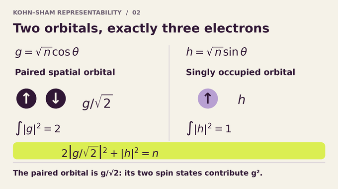
The proof next builds orbitals from the full interacting density. Minimize the weighted angle energy over odd angles, with one electron assigned to the sine component:
A minimizing angle can be folded between zero and above the plane. Define:
Parity makes the orbitals orthogonal. Their squared amplitudes add to . Because has norm squared two, the normalized doubly occupied spatial orbital is , not . This normalization is essential to the three-electron occupation count.
The variational equation supplies a positive multiplier and a common formal potential . In distributional form:
At this stage, “formal” is deliberate. Local regularity does not establish membership in the global admissible potential space.
For a direct normalization check, the paired orbital contributes to the density, and the singly occupied orbital contributes . Their integrals are two and one. On the plane, the sine component vanishes exactly, so the entire interacting density must be carried by the positive paired component.
08. The Weighted Spectral Gap That Makes the Construction Work
Two common-potential equations do not by themselves prove that the occupied orbitals are ground-state orbitals. A lower unnoticed level could invalidate the proposed occupation.
The proof establishes a weighted Poincaré inequality with weight . For a weighted-mean-zero test function , its gradient energy is at least times its weighted squared norm. The full inequality subtracts the weighted mean when it is nonzero.
Odd tests are controlled through the positive ratio in the upper half-space. Even tests require the larger even-sector gap of the zero-coupling operator, together with exterior estimates preventing weighted mass from escaping to infinity. The positivity of later opens a strict interval of forbidden decay rates.
This is a different use of spectral control from the many-body setting in our global spectral-gap explainer. Here it certifies the ordering needed for a density-constrained kinetic search.
Exterior control is essential because convergence on every fixed compact region does not prohibit a sequence of test functions from moving farther away. The strip comparison and localization estimates close that loophole. Without them, the even-sector limiting argument would not establish a global weighted inequality, and the subsequent ensemble certificate would lack its foundation.
09. Why Every Ground-State Ensemble Faces the Same Obstruction
For any three-electron ensemble, the one-particle reduced density matrix satisfies and . The upper bound applies to each spin orbital. A single spatial orbital can hold two electrons because its two spin states are distinct.
Combining this Pauli bound with the weighted gap gives, for every ensemble with density and finite kinetic energy:
The determinant occupying , , and attains equality. It therefore minimizes kinetic energy among all ensembles with that density, including complex spinors and spin coherences.
If an admissible potential represented the density, this determinant would attain the same ground energy. A variational argument then makes an eigenfunction of its one-particle Hamiltonian, forcing . Arbitrary degeneracy cannot evade that identification.
This is the decisive reduction from infinitely many possible ensembles to one candidate potential. It does not assume that all competing states share the constructed orbitals. Instead, equal density fixes their potential-energy contribution, and kinetic minimality forces the constructed determinant into any hypothetical representing ground space.
10. The Final Contradiction: Exponential Decay Versus the Planar Density
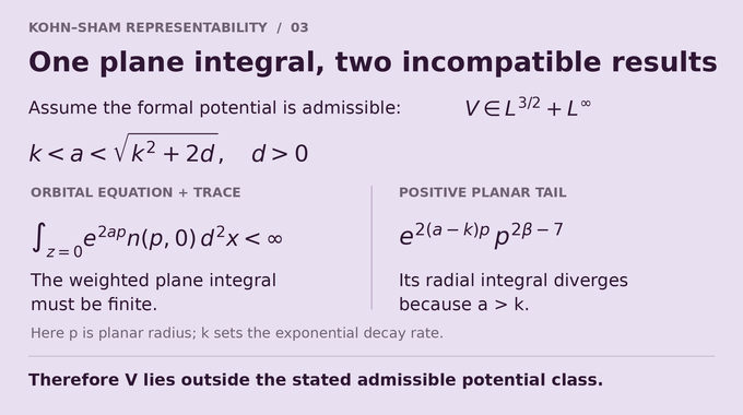
Assume the formal potential belongs to . Translate bounded observation windows toward infinity. The integrable part vanishes locally, while subsequences of the bounded part have weak limits. The density asymptotics and orbital equations force every such limit to equal . No pointwise potential limit is assumed.
Exterior quadratic-form bounds then yield for a rate satisfying . Here controls both the function and its first weak derivatives. The trace theorem transfers weighted square integrability to the median plane.
But oddness gives there, so . Squaring the planar lower bound and including the planar polar-area factor gives:
Since , exponential growth defeats every fixed polynomial power. The same integral must be finite and infinite, completing the contradiction.
The plane itself has zero three-dimensional volume, so its behavior cannot be compared with a bulk density integral without additional regularity. The weighted Sobolev estimate supplies exactly that missing bridge. The trace theorem turns information on a lower-dimensional slice into a legitimate contradiction with the orbital equation.
11. From a Family of Counterexamples to an Exactly Specified Coulomb System
Theorem 6.5 first establishes a family: for every sufficiently large fixed , all sufficiently large integer charges give counterexamples. Section 7 selects one member by fixing and testing auxiliary couplings.
A bad set collects nonregular couplings and failures of sufficient density, multiplier, and angle-comparison tests. The prescription quantifies over every folded minimizing angle. Equation 7.10 defines:
The indicator equals one on the bad set and zero elsewhere. All sufficiently small positive couplings pass, making the supremum finite. The chosen lies outside . These tests use the auxiliary system, not a search over unknown representing potentials.
This is an exact finite nonnumerical specification. Neither a decimal charge nor an effective numerical upper bound is supplied. The physical nuclear separation is , so quoting bohr as the specified separation would misread the scaling.
The sufficient tests form a finite list of conditions, but their definitions use exact spectral, variational, and exterior information. They are not a claimed short numerical algorithm for evaluating the charge. The paper’s achievement here is an unambiguous specification, rather than a chemically realistic parameter choice or a computed molecule.
12. What the Proof Changes and Does Not Change for Exact Kohn–Sham DFT
Corollary 8.1 sharpens the consequence. At the physical density, the ensemble noninteracting kinetic functional has no subgradient in . The ensemble Hartree–exchange–correlation functional has no single potential in that class representing its one-sided first variation along every segment in the common finite-energy density domain.
Here Hartree–exchange–correlation means the interacting ensemble internal-energy search minus the noninteracting ensemble kinetic search. Including Hartree in that definition matters: the corollary concerns this combined functional, with its specified domain and potential dual.
The “every segment” qualification matters. This does not rule out every restricted derivative, distributional potential, spin-dependent formulation, nonlocal operator, or approximate DFT method. Nor does it quantify chemical-energy errors or compare software packages.
For readers following our ionization-conjecture coverage, this is another reminder to separate exact Coulomb statements from practical computational claims. Kohn–Sham representability is an existence question even before approximation enters.
The lasting lesson is specific: interaction can create a physically admissible density that defeats the usual exact noninteracting ensemble replacement in this potential class. Follow Binary Verse AI for research explainers that trace each conclusion through its assumptions, equations, and remaining limits.
Does OpenAI’s proof show that density functional theory is wrong?
No. It establishes a counterexample to exact noninteracting ground-state ensemble representability for a specified class of real, spin-independent local potentials. It does not overturn the Hohenberg–Kohn theorems or demonstrate that ordinary DFT calculations generally fail.
Why do the Hohenberg–Kohn theorems not guarantee Kohn–Sham representability?
They address the interacting density–potential relationship, not whether the same density can be produced by a noninteracting system. That requires a separate existence result.
Can an ensemble of Kohn–Sham states reproduce the constructed density?
Not within the paper’s potential class. The proof excludes every noninteracting ground-state ensemble in that class, including arbitrary ground-space degeneracy and complex spinful states.
Why does the proof use three electrons and two widely separated nuclei?
This construction supplies a paired even orbital and a singly occupied odd orbital, together with a nodal plane and a nonzero interaction-induced density tail. These features permit the asymptotic contradiction.
Are the nuclei separated by bohr?
Not as a specified physical distance. The paper sets in scaled coordinates. The physical separation is , where is a finite integer defined exactly but not numerically evaluated.
What does the proof imply for the exact Kohn–Sham potential and exchange–correlation functional?
It excludes an admissible representing potential for this density and establishes a related obstruction to a full-domain local first variation of the ensemble Hartree–exchange–correlation functional. It does not establish failure for every generalized potential or approximate DFT method.