
A quantum optimizer can improve forever on small test problems without proving it can approach the best possible energy in an infinitely growing system. OpenAI’s September 25, 2026 QAOA proof preprint addresses precisely that gap. The QAOA algorithm, short for Quantum Approximate Optimization Algorithm, alternates problem-dependent interactions with mixing rotations. The manuscript proves that its best limiting expected energy per spin approaches the Sherrington–Kirkpatrick spin-glass optimum, provided system size tends to infinity before circuit depth increases.
For each desired accuracy, suitable finite-depth circuits have angles independent of size and random couplings. That is an expressiveness theorem for a specific model. It supplies neither a practical depth estimate nor a quantum speedup. The important question is how ordinary QAOA gates acquire enough expressive power to reproduce a near-optimal classical calculation.
Table of Contents
1. What Is the QAOA Algorithm, and What Has OpenAI Proved?
The original QAOA construction begins with a uniform superposition of bit strings. A cost operation changes phases according to objective values. A transverse-field mixer rotates qubits, allowing subsequent interference to redistribute measurement probabilities. Repeating this pair times defines a QAOA circuit with cost angles and mixer angles .
In ordinary variational use, a classical optimizer adjusts those angles using measured energies. Our quantum computing and AI guide provides broader context. Here, the proof concerns which energies suitable angles can attain, rather than whether a training loop discovers them.
1.1. QAOA Algorithm: Key Facts
| Feature | Verified Scope |
|---|---|
| Problem | Gaussian zero-field SK model. |
| Main result | Optimal limiting expected energy per spin approaches the Parisi value. |
| Limit order | System size first, then QAOA rounds. |
| Parameters | Deterministic angles independent of size and disorder. |
| Resource guarantee | Finite rounds for every accuracy, without a quantitative depth bound. |
2. The Sherrington–Kirkpatrick Model: The Optimization Problem Behind the Proof
The Sherrington–Kirkpatrick model assigns each spin a value . Every pair interacts through an independent standard Gaussian coupling . In the paper’s maximizing convention, the objective is:
Here counts spins. Positive couplings favor equal signs, negative couplings favor opposite signs. Competing preferences create frustration: three pairwise wishes around a triangle need not be jointly satisfiable. The normalization keeps the optimum proportional to system size.
The positive constant is the limit of the expected maximum divided by . Calling it a ground-state value uses the sign-reversed physical energy. The cost operator replaces each spin by its Pauli operator. The mixer is .
Unlike the sparse interactions in the Mézard–Parisi formula, SK couples every pair. Unlike Heisenberg ferromagnetic ordering, the target here is classical optimization, implemented through quantum dynamics.
3. Why Earlier QAOA Results Could Not Establish the SK Optimum
Fixed-instance convergence allows circuit depth to grow for one particular finite problem. It does not provide a single finite depth that retains a specified accuracy as system size grows without bound.
Earlier work calculated the infinite-size performance of fixed-depth QAOA. The Basso–Farhi–Marwaha–Villalonga–Zhou analysis connected SK performance to large-degree trees and conjectured eventual convergence to the Parisi value. Numerical optimization, later spin–boson representations and semiclassical calculations supported that possibility. Finite-depth data still could not establish the infinite-depth limit.
Numerical convergence cannot substitute for a construction whose parameters are fixed before the system-size limit.
The missing argument had to choose a finite circuit for each accuracy before taking the thermodynamic limit. As in our random 3-SAT threshold explainer, understanding individual finite objects and controlling a limiting random model are separate tasks. Here, the new work builds the required circuit through successive approximations.
4. The Central Theorem: How QAOA Reaches the Parisi Limit
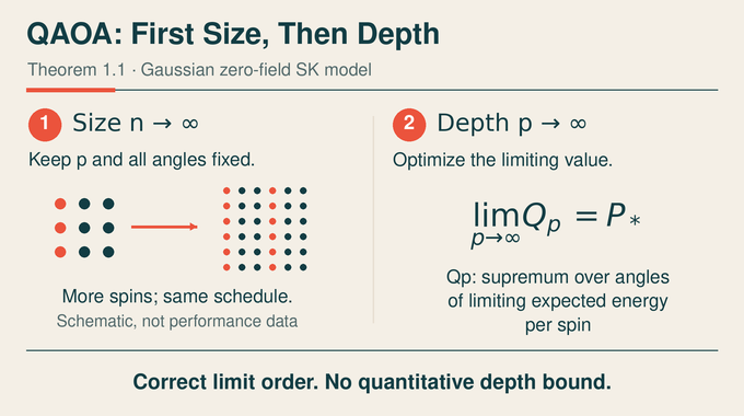
Let denote expected cost per spin after taking at fixed depth and fixed angles. Expectation includes the random couplings and quantum measurement. Let be the supremum of this limiting value over angles. Theorem 1.1 states:
Equivalently, every admits some finite and deterministic angle vectors satisfying . They depend on accuracy, but not on or . This is stronger than allowing parameters to adapt separately to each disorder instance.
This quantifier order permits one circuit to serve an entire growing ensemble. It does not promise that a particular small instance, or every single measurement from that circuit, has energy within the requested tolerance.
Two observations simplify the proof. Measurement produces classical spin configurations, so expected energy cannot exceed the classical optimum. Adding a zero-angle round preserves performance, making nondecreasing. The remaining task is to construct circuits arbitrarily close to the upper bound. Neither a simultaneous size-depth limit nor a finite-size accuracy guarantee follows automatically.
5. From QAOA Circuits to Gaussian Trees and Bosonic Operators
The proof moves to a regular tree of degree , where a fixed-depth circuit accesses only a finite neighborhood. Normalized sums over many centered child calculations develop Gaussian behavior as grows. The fixed-word correspondence identifies the resulting tree energy with the thermodynamic SK energy.
Symmetric Fock space organizes these child states by how many depart from their initial state. Its “particles” count subtree excitations, not additional physical particles or hardware qubits. Creation and annihilation operators encode the limiting Gaussian coordinates.
A root insertion vector records the circuit’s response to a local observable. A root-shift operator places a centered vector into one child while resetting the new root. The limiting energy becomes:
This expression supplies a common comparison space for circuits and classical formulas. Norm approximation controls energy because the root shift has norm one. The proof can therefore track accumulated errors without recalculating every finite graph’s correlations.
6. How Parisi Diffusion Produces a Near-Optimal Classical Formula
The classical target comes from a minimizing zero-temperature Parisi order parameter. Its full-support property means its associated measure has no gap below overlap one. The companion full-support manuscript supplies this property and diffusion identities used by the QAOA argument.
Writing for the spatial derivative of the Parisi value function, the scalar process obeys:
Here is Brownian motion. The scalar function is an order parameter, distinct from the QAOA angle vector. Its diffusion identities express through expected spatial curvature. Stopping before time one and discretizing yields a finite calculation in independent Gaussian variables.
More explicitly, let be that curvature. At a fixed cutoff , the finite discretization builds a rounded output and normalized martingale differences . These are products of an Euler-discretized curvature value and the next Gaussian, rescaled to unit second moment. Define and , where the are independent standard normals and . Their shifted pairing is the bridge to rooted energy:
The mesh limit is taken at fixed . Only afterward does approach one. This order prevents endpoint regularity assumptions from slipping into a finite approximation. The Euler variables approximate the scalar diffusion at finitely many fixed grid times.
An extra Gaussian generates a uniform random threshold. Sign rounding then preserves the terminal gradient as a conditional mean. Products of finite Gaussian coefficients recover the energy and approach the curvature integral. Orthogonality makes these Gaussian coordinates exact in the rooted representation. Appendix A supplies an independent positive-temperature route, followed by the same compilation steps.
7. Turning the Gaussian Formula into Bounded Local Computations
The raw formula is not yet suitable for controlled gates. Its sign output is discontinuous, and intermediate transmitted quantities can be unbounded. The proof smooths the sign, truncates inputs and approximates local functions with finite trigonometric sums. It preserves odd parity, which keeps transmitted outputs centered.
The final local output has the form for a bounded angle calculation . This is useful because a spin rotation can encode precisely that response.
The trigonometric approximation is more than cosmetic. Sines and cosines connect bounded nonlinear calculations to the rotation identities available from quantum controls. Bounding each transmitted column also gives the moment estimates needed when those calculations are reused inside larger operations.
Gaussian labels also assign vertex types. Every aggregation excludes the receiver’s type, ancestor types along its active path and reserved helper types. Refining the partition makes the energy loss small. These exclusions prevent a compiled operation from feeding back into the quantities controlling it. They do not make computations sharing descendant subtrees independent. That distinction is essential to the later commutator estimates.
8. How the Proof Compiles Classical Calculations into Quantum Gates
Theorem 4.1 temporarily permits a longitudinal field formed from independent Gaussian labels. Together with cost and mixer operations, it creates masked local rotations and interactions between selected vertex types. Sign averaging cancels unwanted couplings, while commutator products synthesize new effective generators.
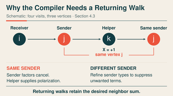
The difficult operation is a neighbor sum of an already defined lower-level calculation. The construction uses receiver, sender and unused helper types. Nested commutators generate walks from receiver to sender to helper and back to a sender.
When the last sender is the original sender, the repeated sender factors cancel. The helper remains polarized in its initial state, leaving the desired contribution. Walks ending at a different sender produce unwanted terms. Subdividing the sender type and retaining pairs in the same subdivision preserves every returning walk while suppressing different-sender contributions in the refinement limit.
The estimates must also control disturbances inside lower calculations, including repeated calls within a surrounding circuit. Compilation therefore proceeds from outer operations inward, fixing tolerances before choosing finite approximations. Small helper probability contributes a controlled energy loss.
This is an existence construction for a finite gate word. It does not provide the optimized logical resource counts discussed in our Claude quantum circuits analysis.
9. Removing Gaussian Seed Controls: The Singular-Echo Construction
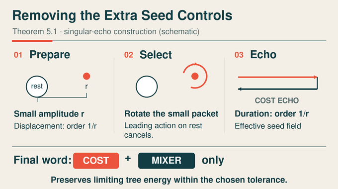
A circuit that still needs random longitudinal fields would exceed ordinary QAOA’s allowed controls. Theorem 5.1 removes them from an already fixed seeded word while preserving its limiting tree energy.
An imperfect cost echo prepares a small component of amplitude with coherent displacement of order . Selective rotations act on this displaced component while canceling their leading action on the much larger remainder. A long cost echo, also of order , amplifies the change into a finite effective longitudinal field.
The construction separates this seed direction from the circuit’s existing Gaussian coordinates, allowing the same effective seed to serve repeated gates. A separate one-particle calculation checks that the energy pairing survives, beyond merely matching Gaussian distributions.
Small norm alone would not make this step harmless: the small component carries a diverging displacement. The proof keeps displaced packets separate from their controlled tails and tracks the root-shift pairing explicitly. That is why matching the seed’s probability law is insufficient to finish the argument.
The parameters are eventually fixed at finite values. The resulting circuit uses only cost and transverse-field mixer pulses, potentially with large or negative angles. Such real-angle existence differs from the finite-gate resource guarantees examined in exact quantum factoring.
10. Completing OpenAI’s QAOA Proof: Error Bounds and a Finite Circuit
Section 6 allocates a requested energy error across the construction. Its bookkeeping makes the order of choices explicit.
10.1. The Proof’s Energy Error Budget
| Stage And Allowance | What the Bound Controls |
|---|---|
| Classical formula: | Approximation to the Parisi target. |
| Helpers: less than | Choose , giving . |
| Seeded synthesis: | Use synthesis tolerance , giving loss . |
| Seed removal: less than | Approximate the fixed seeded word with ordinary gates. |
The ordinary word consequently has energy above . Only after choosing its finite pulse list and every angle does the argument transfer its tree value to SK. Taking the thermodynamic limit while the circuit itself keeps changing would require a uniform estimate that the manuscript does not provide.
11. What the QAOA Proof Establishes for MaxCut
Corollary 1.2 concerns finite simple unweighted -regular graphs with girth greater than . Girth is the shortest cycle length. This condition makes each relevant edge neighborhood tree-like. For sufficiently large , suitable normalized angles give:
Here is the expected fraction of cut edges, and is the chosen accuracy. The actual MaxCut cost angles scale as . The normalized angles and round count are fixed independently of graph size and degree.
For example, requires girth greater than seven in the deterministic graph statement. This illustrates the neighborhood requirement, not a claim that three rounds reach a particular accuracy. Moreover, counts alternating QAOA rounds, not a degree-independent depth after decomposition into two-qubit hardware gates.
The near-optimality comparison is separate: for random regular graphs, system size tends to infinity first, then degree. The optimal-minus-QAOA expected cut gap, multiplied by , becomes arbitrarily small in graph probability. The theorem does not establish optimality for every high-girth graph, arbitrary MaxCut instances or fixed-degree optima.
12. What the QAOA Proof Does Not Establish: Depth, Efficiency, and Quantum Advantage
For developers, the unresolved resource questions determine whether this expressive power becomes useful software. As our quantum query complexity and quantum circuit lower-bound explainers emphasize, performance depends on which resource a theorem actually controls.
12.1. What Remains Unquantified
| Question | What This Manuscript Provides |
|---|---|
| Required rounds | Existence, without a quantitative depth bound. |
| Angle selection | Suitable deterministic angles, without an efficient selection procedure. |
| Finite devices | No quantitative finite-size convergence rate or hardware benchmark. |
| Classical comparison | No proved computational speedup. |
The Lean scope documentation covers supporting Parisi value identities and finite Gaussian approximations, conditional on an admissible minimizer and diffusion, plus full support of admissible minimizers. It does not establish minimizer existence separately or assert the final QAOA circuit-energy convergence theorem. As with any Lean formalization, the checked statement’s scope matters. OpenAI’s mathematics release announcement establishes provenance, not experimental validation.
The QAOA algorithm now has a manuscript-level route to the SK optimum in the specified ordered limit. Turning it into a competitive optimizer still requires depth bounds, angle algorithms and finite-system tests. Hardware studies such as Willow quantum echoes answer a different evidence question. Follow Binary Verse AI’s research explainers and videos to understand what each proof establishes and what the next experiment must test.
What is the QAOA algorithm?
The Quantum Approximate Optimization Algorithm is a variational quantum algorithm that alternates cost-Hamiltonian and mixer-Hamiltonian operations to optimize a target objective. The new proof concerns its limiting performance on the Gaussian zero-field Sherrington–Kirkpatrick model.
Is QAOA a variational quantum algorithm?
Yes. QAOA uses adjustable circuit angles, usually optimized through classical feedback. The paper proves the existence of suitable deterministic angles for the SK limit, not the efficiency of finding them.
What exactly does OpenAI’s QAOA proof establish?
It establishes that optimal expected QAOA energy per spin converges to the Parisi optimum when system size approaches infinity at fixed depth and fixed angles before QAOA depth increases.
Why must system size approach infinity before circuit depth?
That order defines the theorem: it first evaluates each fixed-depth, fixed-angle circuit in the infinite-system limit, then increases depth. Reversing or combining those limits is a different mathematical statement not established by this proof.
Does OpenAI’s QAOA proof establish optimal solutions for MaxCut?
It establishes a leading-order expected cut guarantee for specified high-degree, high-girth regular graphs, together with leading-order optimality for random regular graphs in successive size-then-degree limits. It does not establish universal MaxCut optimality or optimality for every high-girth graph.
Does the proof establish a practical quantum speedup?
No. It provides neither an efficient procedure for determining the required angles nor a quantitative circuit-depth bound, so it does not establish a computational advantage over classical optimization.
Has the complete QAOA proof been formally verified?
Not in the accompanying Lean formalization. It covers supporting SK ground-state value identities and finite Gaussian approximations conditional on an admissible Parisi minimizer and diffusion, plus full support of admissible minimizers. It does not assert the complete QAOA circuit convergence theorem.