
Shuffle a network while keeping every person’s number of connections fixed. The operation is easy. Knowing when the shuffled network has forgotten its starting point was the hard part. The switch chain mixing conjecture asks whether this forgetting always takes polynomially many steps. OpenAI’s September 25, 2026 preprint proves the simple-undirected formulation for every graphical degree sequence: its specified lazy chain reaches total-variation distance at most one-quarter from uniform within steps. The result removes degree restrictions, rather than demonstrating a faster production sampler. Its central insight controls interactions between local updates that look separate but still share edges.
Table of Contents
1. Switch Chain Mixing Conjecture: The Original Problem
Fix labeled vertices and prescribe a degree vector . “Graphical” means at least one simple undirected graph realizes those degrees. Simple excludes loops and multiple edges. Labels matter: vertex 1 must retain its assigned degree, rather than exchange identities with another vertex.
Uniform sampling gives every valid labeled realization equal probability. This supplies a network null model: does an observed pattern survive comparison with graphs having identical degrees? It also connects to approximate counting, a relationship explored in our counting perfect matchings explainer. Sampling graphs with fixed degrees and sampling matchings remain different tasks.
1.1. Switch Chain Mixing Conjecture: Key Facts
| Research source | OpenAI preprint, September 25, 2026; Theorem 1.1 and Corollary 1.2. |
|---|---|
| Input | Any graphical labeled degree vector; the mixing theorem assumes . |
| State space | All simple undirected realizations, with no additional host-edge restrictions. |
| Mixing guarantee | At most proposed steps to total-variation distance . |
| Exact sampling | Unbiased random bits; almost-sure termination; expected polynomial bit cost. |
| Practical evidence | The manuscript supplies proofs, without runtime benchmarks. |
For example, a highly connected vertex can create apparent structure simply because it touches many others. Degree preserving randomization keeps that baseline intact while changing its partners. A comparison against this ensemble asks what degree information alone can explain. It does not establish causation or show that a real network was generated uniformly. The promise concerns distributions rather than a graph’s random-looking appearance.
2. How Edge Switching Randomizes a Graph Without Changing Degrees
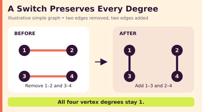
Suppose edges 12 and 34 exist, while 13 and 24 do not. Remove the first pair and insert the second. Each vertex loses one connection and gains one, so every degree survives. Other edges among the four vertices can remain unchanged. A missing old edge or an already present proposed edge makes this particular proposal invalid.
The chain first stays put with probability one-half. Otherwise, it chooses a four-vertex set uniformly and then one of six ordered pairs of distinct perfect matchings uniformly. Each four-vertex complete graph has three perfect matchings, hence six ordered choices of an old and a new matching. A valid proposal executes the switch. An invalid proposal leaves the graph unchanged.
These rejected proposals count as steps. Resampling until a move succeeds changes the transition rule and can change the stationary distribution. Reverse switches have identical proposal probabilities, which makes the uniform law reversible. The explicit holding probability also prevents periodicity. A perfect matching here is merely a proposal on four vertices, rather than the global optimization problem in our maximum cardinality matching analysis.
3. What Does Polynomial Mixing Time Actually Mean?
Write for the finite, nonempty collection of valid graphs and for its uniform distribution. Let denote the transition kernel, so is the distribution after steps starting from graph . Total-variation distance measures the largest probability discrepancy over events, equivalently:
The paper defines the mixing time using the worst starting graph:
A quarter is a conventional accuracy threshold, not a probability that the output graph is “wrong.” Every output already has the correct degrees. The remaining error concerns how often each valid graph appears. Polynomial mixing time means a fixed polynomial bounds the required steps uniformly over inputs. It does not say successive samples are independent or that the bound is tight. For tighter accuracy, the later exponential estimate supplies the additional dependence.
Mixing is a statement about the distribution across repeated runs. Looking at one graph cannot reveal its distance from uniform, and watching one statistic stabilize does not certify all events. The theorem supplies a universal guarantee precisely because such empirical observations can miss a slowly changing feature elsewhere in the state space.
4. The Previous Barrier: Why Existing Proofs Could Not Handle Every Degree Sequence
The Kannan–Tetali–Vempala conjecture grew from work on degree-constrained sampling. Regular undirected graphs, where every degree agrees, received polynomial bounds. Later results covered irregular families under quantitative restrictions. These were substantial guarantees, but did not cover arbitrary graphical vectors.
The unified P-stability theorem broadened the landscape. Roughly, P-stability requires that nearby degree perturbations do not inflate realization counts by more than a polynomial factor across the family. OpenAI’s theorem needs no such family-level hypothesis.
Fu, Qin, and Wang’s binary fixed-margin swap-chain result settled the bipartite formulation. There, a rectangular zero-one matrix records edges between two vertex classes. Prescribed row and column sums encode degrees, allowing a two-row resampling argument.
An undirected adjacency matrix is symmetric. Redistributing one row independently can break that symmetry. The new proof therefore uses updates that change both ends of affected edges consistently, then controls their dependence. It reproves an equivalent three-row inequality from Fu, Qin, and Wang, with attribution. The advance lies in extending the machinery to the undirected obstruction.
5. The OpenAI Proof: The Theorem That Removes the Degree Restrictions
Theorem 1.1 in the switch-chain manuscript states that, for every and every graphical labeled degree vector,
If more than one graph realizes the vector, the spectral gap satisfies:
The gap quantifies the slowest decaying nonconstant mode of the chain. If there is only one realization, no randomization is needed and the mixing time is zero.
“Every” applies within this precise model. The theorem does not establish mixing for arbitrary forbidden-edge hosts, directed graphs, or multigraphs. It also permits disconnected realizations, so imposing an additional connectedness restriction needs separate analysis. Nor does it report a benchmark or an optimal exponent. OpenAI’s mathematics release announcement identifies these papers as results produced by an internal frontier model. The relevant evidence here is the argument and its formalization scope, rather than model branding.
For scale, substituting just ten vertices into the bound already gives two hundred million proposed steps. That arithmetic illustrates how conservative a universal polynomial guarantee can be. The theorem does not identify the slowest actual degree vector, prove this exponent necessary, or compare wall-clock costs against existing graph generators.
6. Pair Resampling: Turning Graph Switches Into Conditional Projections
Fix a vertex pair . Record every edge away from the pair, whether edge exists, and how many neighbors each outside vertex has inside the pair. These fixed data define a conditional collection, called a fiber.
Outside vertices with zero or two neighbors inside the pair have no choice. Those with exactly one are singleton neighbors. If there are singletons and the degree of requires of them, every -element subset is admissible. Uniformly selecting one redistributes these neighbors while preserving every degree. This is an undirected Curveball trade, potentially bundling several individual switches.
Let average a function over its fiber. Define:
Here is the identity operator. Both and are orthogonal projections under the uniform graph measure. Informally, extracts fluctuations erased by resampling pair . The proof studies real functions on graphs rather than trajectories directly. This operator viewpoint resembles the variance-control approach in our common-basis counting explainer, although the underlying state spaces and inequalities differ.
7. The Three-Row Variance Inequality: Controlling Overlapping Vertex Pairs
Two pair updates that share a vertex belong to one three-vertex set. Condition on the graph outside that triple, each outside vertex’s neighbor count inside it, and the number of internal edges. External adjacencies become a three-row binary matrix with fixed margins.
The internal graph needs careful bookkeeping. For one internal edge, an extra column marks its two endpoints. For two internal edges, it marks the center of the resulting path. Empty triples and triangles need no extra column. This encoding preserves the entire conditional space, rather than silently freezing a legal move.
For arbitrary functions of augmented row , the key estimate is:
The proof separates label assignments at fixed block sizes from the fluctuations of those sizes. Transpositions control the assignments, and a conditional-variance argument handles the random counts. The factor two then yields for the sum of pair operators inside triple . The symbol means that the difference has nonnegative quadratic form on every function. Thus overlapping updates receive a usable local bound.
8. The Hardest Barrier: Why Disjoint Pair Resamplings Interfere
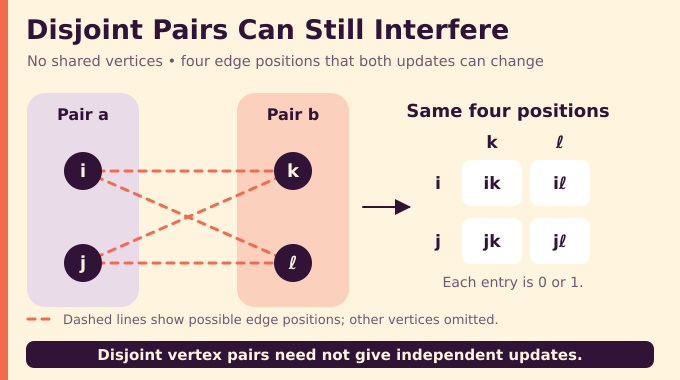
Take disjoint pairs and . Their vertex sets do not overlap, but both updates can change edges , , , and . These four edges form a two-by-two cross matrix. Disjoint vertices do not imply independent operations.
After conditioning on preserved information, most cross-matrix cases factor independently. The difficult case has exactly two present cross edges. There are six such matrices. Two are perfect matchings, one edge in every row and column. The other four concentrate both edges in a row or a column. Row concentration and column concentration cannot occur together.
The remaining dependence between the two conditional data sets has rank at most one. That confines the obstruction to a small correlated component, but an individual interaction can still be negative. Simply discarding every disjoint term would invalidate the proof.
Proposition 5.1 bounds that negative contribution using two directed error projections. Each projects onto a centered indicator that two singleton neighbors were assigned to the same endpoint. Centering subtracts the indicator’s conditional mean. A positive cross-switch term survives alongside these errors. Keeping that positive term is what makes the next cancellation possible.
9. How the Slice Inequality Cancels the Negative Contributions
Return to a fiber: all zero-one assignments with exactly ones among positions, uniformly distributed. This is a uniform subset slice. Let exchange positions and , and let project onto the corresponding centered equality indicator. Lemma 6.1 proves:
The right side measures energy available from exchanging assignments. The left side totals the errors identified for disjoint pairs. Equality indicators are quadratic in the binary coordinates, so their span involves only the degree-one and degree-two components of the slice decomposition. The constant component disappears after centering.
The proof compares eigenvalues on those two components. The transposition operator acts there by and , respectively, while the summed projections have no larger eigenvalues. It separately accommodates degenerate slices, where relevant indicators vanish.
Transferred back to graph fibers, the inequality says the total error energy is affordable from the retained cross-switch energy. Summing over disjoint pair pairs therefore gives a positive-semidefinite operator . This is positivity after aggregation. It does not assert that each pairwise interaction was positive or that dependent updates somehow became independent.
10. From Local Estimates to a Global Spectral Gap
Expanding separates identical, overlapping, and disjoint pair indices. Each vertex pair belongs to triples, yielding the exact bookkeeping identity:
The triple inequalities and positivity of supply the final comparison. Consequently, every eigenvalue of is zero or at least one. A remaining danger is multiple zero modes corresponding to disconnected regions of the state space.
A Havel-based switching argument excludes that danger. Starting from any realization, prescribe the first remaining vertex’s neighbors by highest residual degree, with labels breaking ties. A discrepancy supplies a valid four-vertex switch that installs a desired neighbor without losing previously installed ones. Freeze that vertex and repeat. Every realization reaches the same prescribed graph, proving switch connectivity.
Hence only constant functions lie in the kernel. Let be the unnormalized switch-graph Laplacian, summing differences over distinct switch neighbors. A fiberwise comparison gives . Each switch appears through exactly two pair-trade descriptions. With the stated proposal probabilities, , producing the gap in Section 5. The constants depend on counting proposals as well as successful moves.
11. Deriving the Bound and the Exact Uniform Sampling Corollary
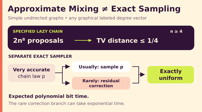
Laziness makes the chain’s eigenvalues nonnegative. The gap therefore gives, uniformly over starting graphs,
There are at most labeled simple graphs. Thus the logarithm of the state-space size contributes only a quadratic factor. Combining that estimate with and allowing integer rounding yields . This controls worst-case switch chain mixing time, not typical observed convergence.
Corollary 1.2 goes further than finite-time approximation. Usually it samples from an extremely accurate chain law . With exponentially small probability , it enumerates realizations and computes a residual distribution satisfying:
The accuracy choice ensures nonnegative residual probabilities. The rare correction branch can take exponential time, but its probability makes its contribution to expected cost polynomial. The sampler uses unbiased bits and terminates almost surely, without a polynomial guarantee on every execution. This resource distinction also matters in our time-space analysis.
11.1. Mixing, Exactness, and Verification
| Lazy switch chain | Approximate uniformity after polynomially many proposals; theorem applies to every graphical vector with . |
|---|---|
| Corrected sampler | Exactly uniform output for any finite graphical labeled vector; expected polynomial bit time. |
| Lean coverage | Mixing bound, exponential total-variation estimate, spectral gap, and connectivity; excludes the separate exact sampler. |
The repository’s Lean scope statement confirms those boundaries. Formalizing selected estimates does not certify an implementation’s speed. As our random 3-SAT threshold explainer also emphasizes, a computational guarantee must be read with its resource assumptions.
An ordinary implementation can use the mixing theorem without implementing the exact sampler. Its output is then approximately uniform at the chosen finite time. Claiming exactness requires the correction construction or another justified exact method. Neither the displayed quarter-distance bound nor a long-looking trajectory eliminates the residual bias by itself.
For developers, preserve the proposal rule and validate the intended state space before using this bound. The switch chain mixing conjecture now has a universal simple-undirected guarantee, while useful practical stopping rules remain a separate engineering question. Follow Binary Verse AI for paper-focused explanations that connect each headline theorem to its mechanism, assumptions, and usable limits.
What is the switch chain mixing conjecture?
The Kannan–Tetali–Vempala conjecture asks whether degree-preserving switch chains mix in polynomial time for every realizable degree specification. OpenAI’s September 25, 2026 preprint proves the simple-undirected formulation for every graphical labeled degree vector, using its specified lazy chain.
How can a switch Markov chain randomize graphs without changing vertex degrees?
A valid switch removes two disjoint edges and replaces them with a different perfect matching on the same four vertices, provided both new edges are absent. Each involved vertex loses one edge and gains one, preserving all degrees and simplicity. Invalid proposals leave the graph unchanged.
What is the mixing time of the switch chain?
For the paper’s specified lazy chain on labeled vertices, the worst-case total-variation mixing time at distance is at most . This is a universal upper bound, not a claim that every instance requires that many steps.
Why was proving rapid mixing for every degree sequence so difficult?
Previous results covered regular graphs and substantial irregular families under additional conditions, including P-stability. Extending the bipartite resampling argument to undirected graphs must preserve adjacency symmetry. Even updates on disjoint vertex pairs can affect the same four edges, creating interactions that require additional inequalities.
How does the OpenAI proof establish polynomial mixing?
It represents neighbor redistribution by conditional averaging projections. A three-row variance inequality controls overlapping pair updates, and a uniform-slice inequality controls the summed errors from disjoint updates. A global operator inequality, switch connectivity, and comparison with individual switches then yield the spectral gap and mixing bound.
Does the OpenAI proof guarantee exact uniform sampling, and is it formally verified?
The paper separately constructs an exactly uniform sampler using unbiased random bits, with almost-sure termination and expected polynomial bit running time. An exponentially rare correction branch can take exponential time. The repository’s Lean scope document covers the mixing bound, exponential total-variation estimate, spectral gap, and connectivity. It excludes the separate exact-sampling algorithm.