
Introduction
A lot of self-supervised vision feels like an elaborate workaround. Two crops, three heads, four losses, and a decoder you throw away the moment you start fine-tuning. This paper tries something refreshingly blunt. It asks: what if we just did prediction, the way language models do, but in the latent space of a vision model?
That idea is next embedding prediction. The authors call the full framework Next-Embedding Predictive Autoregression, or NEPA vision, and they train a plain Vision Transformer with one objective: predict future patch embeddings from past ones, using causal masking, an autoregressive shift, and stop-gradient.
What follows is a practical walkthrough, plus my take on where this fits in the crowded self-supervised landscape, and what I would test next if I had spare GPU budget.
Table of Contents
1. Next Embedding Prediction In One Paragraph
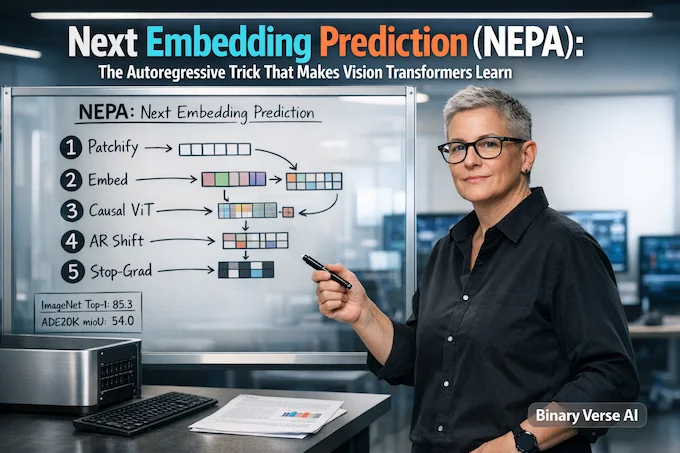
NEPA is simple. Split an image into patches. Map each patch to an embedding sequence z1..zT. Run a causal ViT over that sequence. Train it to predict the embedding of patch t+1 given patches ≤t.
Below is the whole recipe, “parts and purpose.” If you remember nothing else, remember the triad: causal mask, AR shift, stop-grad.
Next Embedding Prediction: NEPA Components Cheat Sheet
| Component | What It Is In NEPA | Why It Matters |
|---|---|---|
| Patch embeddings |
Conv2d patch embedder produces a sequence |
Sets up a learned target space without pixel reconstruction. |
| Autoregressive predictor |
Transformer hθ predicts future embeddings |
Turns pretraining into single-stream autoregressive vision. |
| Causal masking |
Each token attends only to predecessors |
Makes prediction non-trivial, discourages reconstruction shortcuts. |
| AR shift |
Predict t+1, not t |
Prevents identity mapping. |
| Stop-gradient |
Detach targets |
Prevents collapse to constant embeddings. |
| Loss |
Negative cosine similarity of normalized embeddings |
Stable, scalable, easy to implement. |
If you are used to “representations first,” NEPA feels backwards. It is intentionally training a model that predicts, not an encoder that you later repurpose as a frozen feature extractor.
2. Next-Token Prediction, But In Continuous Embedding Space
The mechanics are language-model familiar. Given embeddings z, the model predicts ẑt+1 = hθ(z≤t). The training signal is a similarity loss, not cross-entropy over tokens. They normalize vectors and use negative cosine similarity. Then they stop gradients on the target side so the predictor has something stable to chase.
This is why transformer embeddings matter here. You are not predicting pixels. You are predicting the model’s own internal “currency.” That makes the supervision adaptive, and it also makes the objective feel surprisingly general. If embeddings are the interface, then next embedding prediction is an interface-level objective.
2.1. Transformer Explained, Fast
A quick Transformer Explainer for context. If you have ever Googled “transformer explained” and closed the tab five minutes later, this is the friendly version.
A Transformer mixes information across positions with attention, then refines each position with an MLP. A vision transformer treats patches as positions. A causal transformer adds one rule: no looking ahead. That one rule creates a real prediction problem, and it is exactly what lets a vision transformer behave like a tiny language model over patches.
This is also why people call this “autoregressive” even though the output is a vector. The causal factorization is the point, not the datatype. For more on autoregressive approaches in AI, check out our guide on autoregressive models and their role in modern inference.
3. Algorithm Walkthrough: The Small Details That Make It Work
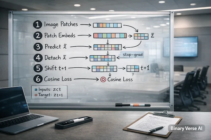
The paper’s Algorithm 1 is almost runnable pseudocode:
- Compute input embeddings z = f(x).
- Predict ẑ = h(z).
- Detach targets, shift by one, normalize, compute cosine similarity loss.
The shift is literal array slicing. pred = ẑ[:, 0:T-1], target = z[:, 1:T]. The loss is then a mean negative cosine similarity across positions.
Two practical notes that are easy to miss if you only read the abstract:
- They evaluate variants under real fine-tuning, not just pretraining loss curves. I like this because collapse and identity mapping can look “fine” until you ask the model to do something useful.
- Reported results use an EMA model with decay 0.9999. That matters if you are trying to reproduce curves.
If you have implemented SimSiam-style losses before, this will feel familiar. If you have not, it is a nice entry point because there are so few moving parts.
4. Why It Does Not Collapse: Stop-Gradient Or Bust
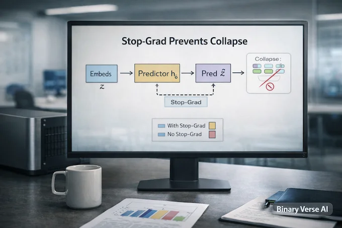
Without stop-gradient, the system can “win” by outputting the same vector everywhere. NEPA detaches the ground-truth embeddings and trains only the predictor side.
They show the failure mode clearly: without stop-gradient, the pretraining loss collapses to −1, and the embeddings become identical. Training dynamics plots frame this as representation collapse.
Here is my mental model. The target embeddings are a moving reference frame, because f is being trained. Stop-grad makes that frame non-reactive per step. The predictor has to align to it. This asymmetry prevents the “everyone meet at the origin” party.
5. Why AR Shift Matters: Copying Is Not Predicting
Remove the autoregressive shift and the objective becomes identity mapping, which gives no meaningful target. After 50k steps, that variant diverges during fine-tuning and fails to converge to a usable model. The paper’s ablation figure says it plainly: without AR shift, training diverges early.
This is also where the “autoregressive” part stops being a metaphor. The shift is what turns similarity matching into next embedding prediction.
6. Causal Masking For Images: Why A Causal ViT Helps
Images do not come with an obvious left-to-right ordering, but causal masking still buys you something. It creates an information constraint, so the model has to build usable context to predict what comes next.
Remove causal masking and the model becomes bidirectional, effectively reconstruction-like. In their 50k-step ablation, that drops fine-tuned ImageNet-1K accuracy from 76.8% to 73.6%.
One subtlety: they keep causality as the default during classification experiments for consistency with the autoregressive formulation, but they also report that enabling bidirectional attention during fine-tuning can improve ImageNet performance when pretraining for 100k steps. For semantic segmentation, they adopt bidirectional attention during fine-tuning by default, because dense prediction needs full spatial context.
So causality is the training discipline. Bidirectionality can still be a fine-tuning convenience. This approach shares similarities with how reinforcement learning influences AI compute scaling in LLMs.
7. Masking Vs MAE: The Surprise Is That Masking Hurts
NEPA tries random masking on the input embeddings while still predicting all targets. Performance drops as masking increases: 78.2% at 0% masking, 76.4% at 40%, 75.7% at 60% (100k steps).
Their explanation is straight. In MAE, masking prevents trivial pixel reconstruction. In this autoregressive setup, prediction is already non-trivial, so masking mostly adds corruption, disrupts sequence structure, and creates train-test mismatch.
My add-on: if your model is learning a patch-to-patch predictive grammar, then masking is like randomly deleting words in the middle of sentences, then acting surprised when the grammar learner gets confused.
8. Modern ViT Hygiene: Helpful, Not The Main Act
The authors also add a modern stability bundle: RoPE, LayerScale, SwiGLU, and QK-Norm, applied at all layers. They describe these as helpful for training but orthogonal to the core framework.
If you want the headlines:
- RoPE is used at all layers and is framed as helping generalization and positional reasoning.
- LayerScale stabilizes training by scaling residual branches with tiny initialized parameters.
- SwiGLU replaces GeLU, with modest improvements, mostly alignment with recent architectures.
- QK-Norm normalizes attention queries and keys to mitigate gradient explosion or collapse.
Their training dynamics figure highlights LayerScale stabilizing optimization and QK-Norm suppressing gradient explosion.
I read this section as a pragmatic message: if you want next embedding prediction to scale, you treat it like any other scaling problem. You add the stability tricks that the community has already paid for. For context on AI efficiency and scaling, explore our analysis of AI efficiency and algorithmic laws in hardware scaling.
9. Results: What “Competitive” Means Here

Now the part that made people look up from their decoders. Pretrained on ImageNet-1K without labels, then fine-tuned, NEPA reaches 83.8% top-1 (ViT-B) and 85.3% (ViT-L). It transfers to ADE20K semantic segmentation at 48.3 mIoU (ViT-B) and 54.0 mIoU (ViT-L).
The comparison table groups NEPA with methods like MoCo v3, BEiT, DINO, MAE, and JEPA, and it also makes a point about simplicity: NEPA uses no decoder and one forward pass per step in that table. On ADE20K, NEPA trained on ImageNet-1K is competitive with the listed baselines trained on the same data.
This is where I inject my “experienced reader” caution. ImageNet top-1 is a crowded leaderboard, and lots of things can shift numbers by a few tenths. What matters is that a minimalist autoregressive objective does not get embarrassed. It lands in the same neighborhood as the heavyweight self-supervised pipelines. When comparing model performance, you might also find our LLM pricing comparison guide helpful.
9.1. Key Numbers At A Glance
Next Embedding Prediction: NEPA Knobs And Outcomes
| Knob | Outcome | Evidence |
|---|---|---|
| Remove AR shift |
Breaks Fine-tuning fails | Not provided |
| Remove causal masking |
Worse 73.6% vs 76.8% top-1 (50k) | Not provided |
| Remove stop-gradient |
Collapses Loss collapses to -1 | Not provided |
| Random masking ratio |
Drops 78.2% (0%), 76.4% (40%), 75.7% (60%) | Not provided |
| ImageNet top-1 |
Headline 83.8% (B), 85.3% (L) | Not provided |
| ADE20K mIoU |
Transfers 48.3 (B), 54.0 (L) | Not provided |
| Linear probing |
Weak 11.3% (last), 14.1% (avg) | Not provided |
10. What The Model “Looks At”: Semantics Shows Up In Attention
The paper’s attention maps are the antidote to “patch order is nonsense.” When predicting, attention is often long-ranged and object-centric, allocating most weight to regions semantically related to the query patch.
They also compute embedding similarity maps by comparing the predicted next embedding to all patch embeddings in the same image. The predicted embedding is most similar to patches belonging to the same object or semantic region, with unrelated background much lower.
This matters because it suggests the model is learning global dependencies, not just local textures. The authors explicitly interpret the attention patterns as forming global, semantically meaningful dependencies between patches. For more on embedding techniques, see our comprehensive EmbeddingGemma guide for on-device RAG.
11. Criticisms From Threads: What Is Actually Different
The “is it new” argument is mostly taxonomy. NEPA sits next to CPC, GPT-like vision models, AIM, and JEPA, but the implementation choices are distinct.
- Versus CPC, it is not contrastive, and the Transformer predictor is the main learned object. It regresses the next embedding without negatives or a contrastive head.
- Versus iGPT and AIM, it shares the causal prediction idea but works fully in continuous embedding space and avoids pixel-space targets, tokenizers, and language heads during pretraining.
- Versus JEPA, it keeps the latent prediction goal but simplifies to a single embedding layer and an autoregressive Transformer predictor, no asymmetric branches and no extra head.
So the “new” part is not the vibe. It is the minimalist bridge between next-token training and a vision transformer. To understand how this compares to recent coding models, check out our reviews of Qwen3 Coder and the best LLMs for coding in 2025.
12. Limitations, My Expert Take, And What To Try Next
Two limitations are worth stating plainly. First, linear probing is poor: 11.3% top-1 using the last embedding, 14.1% using the average. The authors argue this is expected because the probed representation is very close to the embedding layer, so you are not really measuring the predictor’s full capacity.
Second, failure cases show up in physically tricky scenes: reflections, shading, shadows, and scenes with many small or overlapping objects.
My take is optimistic but specific. Next embedding prediction is a clean objective, and cleanliness is leverage. It makes ablations interpretable, and it makes extensions obvious.
If I had a week to push this forward, I would do three things:
- Patch order experiments. Raster order is a convenience, not a principle. Try Hilbert curves, spirals, and random fixed permutations, then measure both accuracy and attention structure.
- Readouts from deeper states. If probing shallow transformer embeddings fails, probe later-layer hidden states, or train a light readout that taps the predictor’s internal features.
- Multimodal and generative coupling. The paper frames embeddings as a “common currency” across modalities, and suggests coupling NEPA with an image decoder or diffusion generator for synthesis or editing.
That last point is the big one. If embeddings really are a shared interface, then next embedding prediction is not just an ImageNet trick. It is a general way to train predictors that can plug into generation later. For insights on how agentic AI systems leverage similar principles, explore our guides on agentic AI tools and frameworks and agentic AI versus generative AI.
So here is the CTA. Pick one of the three experiments above and run it. Post the curves and the failure cases, especially the weird ones. Then send me what you found. The fastest path to insight in this field is still the same: take a simple idea like next embedding prediction, break it in an interesting way, and learn from the repair. If you’re working with advanced models, you might also benefit from understanding Claude Sonnet 4.5’s capabilities and LLM inference optimization techniques.
What does autoregressive mean in machine learning?
Autoregressive means the model predicts the next step using only previous steps. In text, it predicts the next token from earlier tokens. In vision, an autoregressive vision setup predicts the next patch representation from earlier patches, which creates a real “no peeking ahead” prediction problem.
Is ChatGPT an autoregressive model (and why does that matter for NEPA)?
Yes. ChatGPT is trained to predict the next token given prior tokens, which is autoregressive. That matters for NEPA because next embedding prediction borrows the same training instinct, predict what comes next, but swaps discrete tokens for continuous transformer embeddings produced from image patches.
What does ViT stand for in machine learning?
ViT stands for Vision Transformer. It treats an image like a sequence by splitting it into patches, embedding each patch into a vector, and then running Transformer layers over that sequence. A causal ViT adds a causal attention mask so each patch only attends to earlier patches.
What are embeddings in transformers, and what is their purpose?
Embeddings are dense vectors that represent inputs in a form the Transformer can process. In a vision transformer, patch embeddings represent image patches. In next embedding prediction, these embeddings become the prediction target, the model learns to forecast future embeddings, not pixels, which can simplify training and keep the pipeline lightweight.
What is the SimSiam method, and why does NEPA use stop-gradient?
SimSiam is a self-supervised method that prevents representational collapse by stopping gradients through one branch of the network. NEPA uses the same idea, stop-gradient on the target embeddings, so the model cannot “cheat” by making all embeddings identical. It forces learning a real predictive mapping.