TTT E2E: 128K Context Without the Full KV Cache Tax (2.7× Faster Than Full Attention)

Introduction

Long prompts feel like a superpower right up until you pay for them. You paste in 80K tokens of logs, code, or chat history, and the model spends the next few seconds doing what looks like “thinking,” but is mostly bookkeeping.

That bookkeeping is the KV cache. It’s also why long context llm features often ship with a latency asterisk. In full attention, every new token scans keys and values from all previous tokens, and the per-token cost grows with context length. If you’ve ever wondered why 128K context can feel slower than a human reading, that’s your answer.

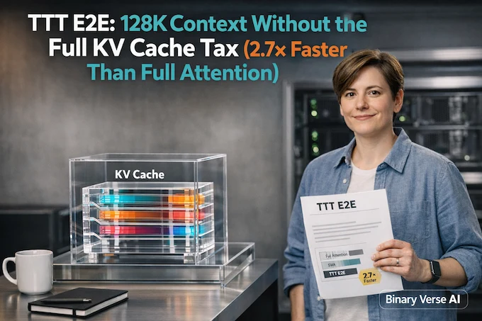
TTT E2E takes a different stance: stop carrying a lossless record of the whole past. Read the context, then compress what matters into a lightweight internal state by continuing next-token training during inference. The paper’s headline is sharp, constant inference latency with respect to context length, reported as 2.7× faster than full attention at 128K on an H100.

This is not a “new attention trick.” TTT E2E is closer to a systems idea than a module idea. It’s inference-time learning with production-shaped constraints.

1. TTT E2E In One Paragraph: The 128K Problem It Targets

Full attention gives you near-perfect recall, but it does it by scanning an ever-growing KV cache, which becomes expensive fast. Sliding-window attention cuts the cost by limiting what you attend to, but it also limits what you can use.

TTT E2E threads the needle, and it does it in a way that keeps the rest of the stack familiar. It keeps a standard Transformer skeleton with sliding-window attention for local detail, then performs small gradient updates on next-token prediction over the context so the model can carry forward a learned summary in its weights. The result is a long-context strategy that aims for linear prefill and constant decode, rather than a KV cache that scales with length.

Table 1. The Fast Decision Summary

TTT E2E is a trade, not a cheat. It buys lower memory traffic by spending compute on learning.

One detail that made me take this seriously: the authors observe that even when you run it “on top of” full attention, the approach can still improve test loss, and the gap between it and a sliding-window baseline stays similar across window sizes. That suggests TTT E2E is not just patching over what sliding windows remove, it’s adding a different kind of capacity.

2. Why Full Attention Gets Punished At 128K

Here’s the kv cache explained version that matches what you see in practice.

A Transformer stores key/value vectors for every prior token. During decoding, each new token attends over that cache. As context grows, the cache grows, and the scan grows. That turns llm kv cache from a helpful optimization into a dominant cost center.

The paper spells out the mechanism: full attention must scan keys and values of all previous tokens for every new token, and the cost per token grows linearly with context length.

With TTT E2E, the other punchline is complexity. In the method section, full attention is summarized as O(T²) prefill and O(T) decode. TTT-style inference targets O(T) prefill and O(1) decode.

That’s why “kv cache llm” problems show up as both latency and memory issues. You either wait longer, or you cut batch size, or you do both. This is llm memory management, except the memory is not your laptop RAM, it’s your GPU’s most precious resource.

3. The Core Idea: Long-Context LM As Continual Learning

Most long-context work is framed as architecture design. The paper flips that framing. It treats long-context language modeling as continual learning, not a new module hunt. Call it continual learning ai, but scoped to one prompt and one moment.

The intuition is surprisingly human: you don’t remember every sentence from your first ML lecture, but you carry forward the compressed understanding. The introduction makes that contrast explicit, humans improve with experience despite imperfect recall, while Transformers struggle partly because they aim for near lossless recall.

This is what “test time training llm” should mean when you talk about this paper. Not a generic fine-tuning session, but inference-time learning that is tied to the specific prompt you are reading.

It also clarifies test time training vs fine tuning. Fine-tuning adjusts a global model for everyone. TTT adapts the model for this one prompt, right now, as part of inference time machine learning.

4. How TTT E2E Works At Test Time

TTT E2E starts with a clean split: prefill (read the context) and decode (predict the next token). Then it adds learning steps during prefill.

4.1 The Update Loop

The loop is simple:

• Predict next tokens over a chunk of the prompt.
• Compute the standard next-token loss.
• Take a small gradient step.
• Repeat for the next chunk, carrying forward updated weights.

Those updated weights are the compressed memory. Instead of dragging a massive KV cache through decode, you carry forward a compact learned state.

In their implementation, this “memory” is not a vague metaphor. It is literally parameter space devoted to fast updates. In one ablation discussion, they contrast a variant that updates smaller multi-head MLPs with a final version that increases effective state, reporting a 5× larger hidden state and about half the prefill latency on H100 in that comparison. That’s a clean reminder that in TTT E2E, memory capacity is tied to which layers you allow to move, and how much you let them store.

4.2 Why Sliding Windows Matter

If you only rely on weight updates, you lose crisp local detail. The final method keeps sliding-window attention, then uses TTT to handle longer-range compression.

Mini-batches introduce a constraint: the model must remember enough inside the batch for the gradients to make sense. For main results at T = 128K, the paper sets window size k = 8K and mini-batch size b = 1K, and emphasizes k ≥ b for within-batch context.

If you like taxonomy, you can also view this through the lens of fast weights. The paper explicitly connects test-time training to fast weights, where inner-loop weights act as “fast” state and outer-loop weights act as “slow” parameters. That framing helps because it replaces mystical language with engineering language: you are allocating a fast-changing state channel, then learning how to write to it.

4.3 Why b = 1K Is A Practical Default

Ablations show the uncomfortable truth: larger b can hurt performance, while too-small b hurts hardware utilization and stability. That’s why b = 1K becomes the default.

This is the most “engineer-coded” part of the method. The math matters, but the schedule matters just as much.

5. Why It’s End-to-End Twice

TTT E2E is “end-to-end” at test time because the inner loop optimizes the same next-token prediction loss the model already cares about.

It’s also “end-to-end” at training time because the outer loop trains the initialization to be good after those inner-loop steps. The introduction describes the bi-level setup: run inner-loop TTT on each sequence, then optimize the post-TTT loss across sequences using gradients of gradients.

If you want a mental model, it’s “teach the model how to learn quickly from context,” not “hope it learns.”

6. Stability And Forgetting: What They Freeze, What They Update

Inference-time learning sounds scary until you notice how conservative the updates are in TTT E2E. During TTT, they freeze embeddings, normalization, and attention layers because updating them destabilizes the outer loop. Only MLP layers are updated in the inner loop.

They also pick a storage-versus-compute point by updating only the last quarter of blocks by default, based on ablations.

This is how you get a method that behaves more like “structured adaptation” than “random drift.” It is also why the approach fits naturally into conversations about llm memory, because the “memory” is now constrained, localized, and trained for.

The “two MLP layers per block” detail is easy to skim past, but it matters. If you’ve ever debugged a model that catastrophically overwrote a feature, you know why. The idea is to give the model a stable lane for pre-trained knowledge, while a separate lane takes the fast updates from the current prompt. It’s the simplest version of “don’t scribble on your only copy.”

7. The Headline Result: Constant Latency At 128K

For TTT E2E, the paper’s key speed claim is straightforward: it has constant inference latency regardless of context length, reported as 2.7× faster than full attention for 128K context on an H100. That is the practical promise. Long context stops being a bill that grows with every extra paragraph.

Quality matters too. The Figure 1 caption claims the method maintains an advantage over full attention at longer context lengths, while several baselines worsen as context grows. If you’re building for long prompts, those two curves, loss and latency, are the whole story.

The caption’s “loss Δ” phrasing is also worth understanding. They compute loss differences relative to a full-attention Transformer, which makes the flat zero line the baseline and highlights how other methods drift as context grows. In that framing, TTT E2E is presented as keeping its advantage even at 128K, instead of fading with length.

8. The Hype Questions, Answered Like An Adult

8.1 “Is This Brain Memory?”

It’s weights as evolving state, optimized by gradients. It will store what helps prediction, not what you personally label as “important.”

8.2 “Does It Forget Stuff?”

Forgetting is a real concern, which is why the inner loop updates only MLP layers and avoids touching the fragile parts of the network. The design also limits how much of the stack is updated by default.

8.3 “Is It Cheaper, Really?”

In the 128K regime, constant decode can dominate. In short-context training, the paper is candid that training latency is a limitation because gradients of gradients are less optimized than standard training.

9. Comparisons People Will Google

Long-context methods differ mainly in where “memory” lives, and TTT E2E is the clearest example of “learned state” in the list:

• Full attention stores it in a growing KV cache.
• RNN/SSM families store it in a fixed state.
• Sliding windows store it locally.
• TTT-style methods store it as learned fast weights.

Figure 1’s baseline list includes sliding-window attention, hybrid variants, Mamba 2, Gated DeltaNet, and TTT-KVB.

When people ask “where do Titans or Nested Learning fit,” the paper groups them near TTT-KVB style hybrids, which combine TTT-MLP layers with key-value binding ideas and sliding-window components. The larger point is that the design space is not one line from attention to recurrence. It’s a grid of choices about state, update rules, and what you freeze.

Table 2. Scaling Cheatsheet

This framing also helps with “RAG vs long-context LLM.” RAG keeps memory outside the model and fetches it. Long-context keeps memory inside the prompt and pays the KV cache tax. TTT-style approaches try to migrate some of that memory into compact learned state during use.

10. How To Run The Code Without Losing Your Mind

The paper states the experiments can be reproduced with the public repository and datasets, which makes TTT E2E unusually testable for a fresh idea. The repo is JAX-based and expects a modern CUDA stack.

10.1 Setup

1. Install uv:

curl -LsSf https://astral.sh/uv/install.sh | sh

2. Download datasets (examples):

gcloud storage cp -r gs://llama3-dclm-filter-8k/ llama3-dclm-filter-8k
gcloud storage cp -r gs://llama3-books3/ llama3-books3

3. Point configs/deploy/interactive.yaml (or submitit.yaml) at your local paths.
4. Set W&B fields: training.wandb_entity, training.wandb_project, training.wandb_key.

10.2 Run

Interactive:

uv run --exact train \
  +deploy=interactive \
  +experiment=125m/pretrain/pretrain-125m-e2e \
  training.wandb_entity=my-entity \
  training.wandb_project=my-project \
  training.wandb_key=my-key

Slurm:

uv run --exact train \
  +deploy=submitit \
  hydra.launcher.nodes=4 \
  +experiment=125m/pretrain/pretrain-125m-e2e \
  training.wandb_entity=my-entity \
  training.wandb_project=my-project \
  training.wandb_key=my-key

11. Replication Tips: Six Failures You Can Predict

1. Version mismatch (CUDA, cuDNN, NCCL). Fix this first.
2. Requester Pays surprises when pulling from GCS.
3. Hydra overrides not applied, print the resolved config.
4. W&B keys missing, training dies early.
5. OOM during prefill, start small and scale.
6. Bad throughput, the defaults exist for a reason, k = 8K, b = 1K, and k ≥ b keeps within-batch context usable.

This approach is the kind of idea that feels obvious five minutes after you understand it. Of course long context should be compression, not perfect recall. Of course the model should learn from the prompt while it reads it.

Now do the only thing that matters with the idea in mind. Reproduce Figure 1. Measure latency at your context lengths. Compare against your current stack. Then decide where inference-time learning fits in your product roadmap, whether as a replacement for brute-force KV caching, or as a complement that turns your long prompts into something closer to durable, compact memory.