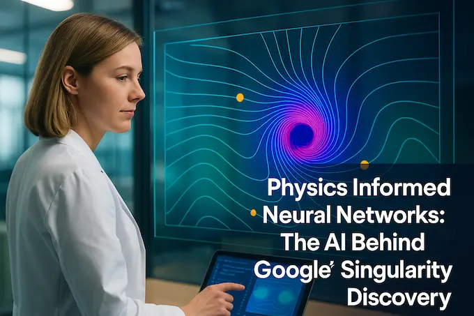
You do not often see a centuries-old math question give way in a single week. Yet that is what happened when a DeepMind-led team revealed new families of unstable singularities in fluid equations. If you care about AI in fluid dynamics, this is the kind of result that resets the map. The secret was not a bigger supercomputer. It was a smarter way to search, one that builds physics into the network itself. That method, physics informed neural networks, turned a seemingly impossible needle-in-a-haystack search into a reproducible workflow and, in the process, pushed accuracy to the brink of machine precision.
Table of Contents
1. What Are Physics Informed Neural Networks
Let’s start with a plain description. A standard neural net learns from data. A physics informed neural networks approach learns from data and from the governing equations. Think of it as teaching with lab notes and with the laws of nature. In practice, physics informed neural networks minimize two things at once. They fit any available observations and they minimize the residual of the partial differential equation, the amount by which the candidate solution violates the physics. Because the equations act like a constant supervisor, physics informed neural networks won’t “hallucinate” unphysical answers as easily, and they can work even when you have little or no labeled data.
There is another benefit. When you embed structure, you compress the hypothesis space. Physics informed neural networks inherit conservation laws, symmetries, boundary behavior, and decay at infinity right in the architecture. That inductive bias turns a messy global search into a guided walk. For problems where the physics is strict, like AI for partial differential equations (PDEs), the difference is night and day.
2. Why Unstable Singularities Matter

Singularities are points where smooth solutions blow up in finite time. They matter because the Euler and Navier-Stokes equations are the backbone of fluid mechanics. If those equations can produce infinite gradients from nice initial data, that signals a fundamental limit in what the equations can predict. Stable singularities are the easy ones to find. Unstable singularities are the delicate, knife-edge profiles that require initial conditions tuned with extreme precision.
For foundational questions about the boundary-free 3D Euler and Navier-Stokes equations, many experts expect only unstable ones to exist. That makes them the real prize and the hardest target. The DeepMind-led work reports the first systematic discovery of unstable families across multiple fluid models, and it does so with accuracy suitable for computer-assisted proofs.
3. How The Discovery Worked, In Human Terms
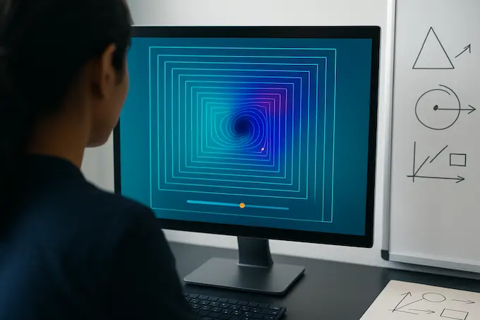
The team did not time-step a turbulent flow and hope it exploded. They searched for self-similar solutions directly. Self-similarity rescales space and time around the blow-up point so that a dynamic event becomes a stationary profile in new coordinates. That reduces a runaway movie to a still frame. Then they asked physics informed neural networks to find a profile and a scaling rate λ that make the self-similar equations hold everywhere. The network did not learn arbitrary fields.
It learned fields constrained to be smooth, to have the right symmetry, and to decay with the right power law at infinity. A Gauss–Newton optimizer and a multi-stage refinement scheme then drove the residual down by orders of magnitude. For some cases, the residual landed near the double-precision round-off floor. That is the level you need for rigorous computer-assisted mathematics.
4. What Exactly Was Found
The team reports unstable self-similar solutions in three settings that map onto big questions in AI in fluid dynamics and mathematical analysis:
- CCF model (Córdoba–Córdoba–Fontelos), a 1D toy that mirrors mechanisms in Euler and Navier-Stokes.
- Incompressible Porous Media (IPM) with a boundary.
- Boussinesq with a boundary, which is mathematically analogous, up to small terms, to the axisymmetric 3D Euler equations.
They list stable and multiple unstable branches along with the blow-up scaling λ for each branch. They also show a simple linear pattern when you plot inverse scaling rate against instability order for IPM and Boussinesq. That pattern suggests where higher-order branches should live, which turns guesswork into a roadmap for future searches. Residuals reach roughly 10⁻⁸ to 10⁻⁷ for IPM and Boussinesq branches, and near 10⁻¹³ for the CCF stable and first unstable branches after refinement.
4.1 A Few Of The Actual Unstable Singularities
Below are concrete examples reported by the authors. These λ values characterize how fast the fields blow up in the self-similar frame.
| Equation | Solution Order | λ (Scaling Rate) |
|---|---|---|
| CCF | 1st Unstable | 0.6057337012 |
| CCF | 2nd Unstable | 0.4713248639 |
| IPM (with boundary) | 1st Unstable | 0.4721297362 |
| IPM (with boundary) | 2nd Unstable | 0.3149620267 |
| Boussinesq (with boundary) | 1st Unstable | 1.3990961222 |
| Boussinesq (with boundary) | 2nd Unstable | 1.2523481636 |
These are taken from the discovery tables and figures in the paper. They demonstrate the existence of multiple unstable branches for each system and the rising hierarchy across orders.
5. Why Classical Methods Struggled, And Why PINNs Helped
High-resolution simulation can catch a stable blow-up. It won’t usually land on an unstable one. Any tiny numerical wobble kicks the trajectory off the unstable manifold. Continuation methods fail when the admissible solutions are isolated rather than part of a smooth family. Regularization can stabilize an event, but then you have to justify the link back to the original equations.
The team’s workaround was to pose the search directly in the stationary, self-similar frame and to build a model where the physics is not an after-thought. Physics informed neural networks supplied the function approximator with the right symmetry and decay. The optimizer targeted the physics residual, not just a fit to snapshots. The result is a discovery engine for vanishingly narrow targets.
Two details are worth calling out:
- Architectural bias. The fields are modeled by compactifying infinite domains to finite ones, using explicit “solution envelopes” that enforce symmetry and asymptotic decay. This lets the network spend its capacity on the real structure rather than learning basics like oddness in y1y_1 or a 1/(1+λ)1/(1+\lambda) decay power. That is a natural role for physics informed neural networks.
- Second-order optimization and multi-stage training. A full-matrix Gauss–Newton method, with clever stochastic estimation of curvature, converged far faster than Adam and L-BFGS and, more importantly, reached residual levels those first-order methods did not. A second network then learned the error of the first, pushing accuracy several orders further. This upgrade was decisive. It is a reminder that physics informed neural networks benefit not only from better loss design, but also from serious numerical optimization.
6. What This Means For AI In Scientific Discovery
The point is not that physics informed neural networks will replace every solver. The point is that they open doors that standard pipelines leave closed. Here, AI in scientific discovery looks like a conversation between mathematics and computation. Self-similar analysis narrowed the search space. Physics informed neural networks gave a flexible yet constrained representation. High-precision numerics supplied the last bit of accuracy that pure deep learning seldom reaches. The combined effect is new objects of study that carry enough precision for proof, not just a nice plot. In that sense, this work belongs in the growing stack of computer-assisted mathematics, where symbolic insight and numerical rigor meet modern ML.
There is also a forward arc. The Navier-Stokes Millennium Prize asks whether smooth initial data can produce finite-time blow-up in 3D. One proposed path is to build a hierarchy of self-similar profiles with increasing instability and show how viscosity stays subdominant on the blow-up time scale. The families reported here, with a simple empirical law for how λ scales with instability order in IPM and Boussinesq, point to a recipe. That is not the final word. It is a confident step.
7. A Hands-On Guide For Builders

If you want to try this yourself, start small and structure first. The workflow below generalizes far beyond fluids, and it respects your time.
7.1 Frame The Problem In Self-Similar Coordinates
When a blow-up is likely self-similar, the right coordinates turn time evolution into a stationary profile. That converts unstable chasing into steady solving. It is the perfect setting for physics informed neural networks. You decide the rescaling, write the transformed equations, and derive any algebraic relationships, like the link between λ and a velocity gradient at the origin. Then you let the learner search over admissible λ values.
7.2 Encode The Physics In The Model
Use symmetry and decay as architecture, not as a regularizer alone. Wrap your network outputs in analytic envelopes that force oddness, evenness, periodicity, or specific power-law decay at infinity. Compactify unbounded domains so your collocation grid fits in a box. This is where physics informed neural networks shine. They reward you for making the right things easy and the wrong things impossible.
7.3 Optimize For Accuracy, Not Just Fit
Go beyond first-order optimizers. Curvature helps, especially as you push residuals into the 10⁻⁸ to 10⁻¹³ range. Multi-stage training can turn one very good solution into an excellent one by learning the remaining error field. With physics informed neural networks, the loss landscape improves when you include derivative residuals, not just the zero-order residual. Sampling also matters. Adaptive collocation that focuses on high-residual regions can cut training time and improve convergence.
7.4 Tooling
You can build physics informed neural networks in general frameworks like PyTorch or TensorFlow. If you prefer batteries included, look at libraries that support PDE loss construction and collocation workflows. NVIDIA Modulus and DeepXDE are popular choices. Start with a tiny model, verify symmetry and decay on a coarse grid, then scale the network and the grid together. Keep a validation script that reports maximum residuals across derivative orders. Treat that script as your unit test for the physics.
7.5 Where Else To Point This
Physics informed neural networks are already useful for inverse problems in materials, for data-scarce models in climate, and for speeding up solvers by providing good warm starts. They are also natural for medical flow modeling, where AI in fluid dynamics must honor conservation and realistic boundary conditions. Anywhere you are solving or designing with PDEs, physics informed neural networks can act as a bespoke function approximator that refuses to break the laws.
8. Beyond Fluids: Breadth Without Hype
The same pattern you saw above generalizes well.
- Material science. Stress and strain models with limited sensor data benefit when physics informed neural networks bake in constitutive laws and geometry.
- Climate modeling. Hybrid models improve skill when the learned parts cannot violate energy budgets or known transport constraints.
- Medical imaging and flow. Blood flow, porous perfusion, and boundary-constrained transport are ripe for physics informed neural networks that are both data-efficient and physically faithful.
- Operator learning, next to PINNs. Neural operators like FNO and DeepONet can generalize across parameter families. When you need a single high-fidelity solution tied to strict constraints, physics informed neural networks remain a sharp tool. When you need fast surrogates across many conditions, pair operators with physics-aware losses.
The healthier view is not either-or. Use physics informed neural networks where the physics is your friend, and call in operators when you need speed and parameter sweeps. In both cases, keep the physics in the loop.
9. The Payoff: A New Rhythm For Proof-Grade Discovery
This study is a clear signal. With the right inductive biases and numerics, physics informed neural networks can do more than interpolate. They can discover target objects that analysts care about and deliver them at a precision compatible with proof. The workflow is honest about tradeoffs. You will not get automatic miracles. You will get a principled search procedure that respects the equations and scales to the accuracy that math demands. That is what a modern scientific method looks like when AI in scientific discovery meets deep domain expertise.
10. Closing Thoughts And A Call To Action
If your team works on PDE-governed systems, set up a small strike team next week. Pick one problem where you suspect self-similar structure or strict constraints. Build a compactified domain. Wrap symmetries and decay into the network head. Train a baseline with a residual-only loss. Then add derivative residuals, adaptive collocation, and a second-order optimizer. Use physics informed neural networks as the spine of the effort. Share your validation script, not just plots.
If you find a candidate solution with a tiny residual, publish the profile and the λ estimate so that computer-assisted mathematics can do its part. The combination of human insight and physics informed neural networks is no longer a curiosity. It is a practical path to results that stand up to scrutiny.
This article references the DeepMind-led research announcing the systematic discovery of unstable singularities and the methodology that made it possible.
1) What Are Physics-Informed Neural Networks (PINNs)?
Answer: Physics informed neural networks are neural nets trained to fit data while also satisfying the governing equations of a system, usually partial differential equations. In practice, a PINN minimizes standard data error and the PDE residual so its predictions obey the physics.
2) How Do PINNs Work Differently From Standard Neural Networks?
Answer: Standard models learn only from examples. A physics informed neural networks approach adds a physics loss that penalizes violations of the PDE and boundary or initial conditions, which guides learning even with sparse data and reduces unphysical outputs. Implementations often include automatic differentiation to compute residuals efficiently.
3) What Are The Main Applications Of PINNs?
Answer: Physics informed neural networks are used for forward and inverse solutions of PDEs in fluid dynamics, heat and mass transfer, electromagnetics, materials, and biomechanics. They also serve as fast surrogates and for parameter identification when measurements are limited. Libraries and docs highlight cavity-flow tutorials, multi-physics setups, and end-to-end inverse problems.
4) Can PINNs Solve Problems That Traditional Methods Can’t?
Answer: PINNs don’t replace classical solvers across the board, yet they can find or refine solutions that are hard to capture numerically, such as delicate self-similar blow-ups and data-scarce inverse problems. Recent work used PINN-style training to uncover new families of unstable singularities in fluid equations, a case where precision and physics constraints were decisive.
5) Are There Any Open-Source PINN Libraries Or Tutorials To Get Started?
Answer: Yes. Popular options include DeepXDE for general PINNs in Python, NVIDIA Modulus for industrial-scale PDE workflows and tutorials, and NeuralPDE.jl in Julia for automatic PINN solvers and operator-learning paths. Each provides docs, examples, and starter code.