

Introduction
Most generative models feel like they’re doing the same ritual: start with noise, take many tiny steps, hope you land on something beautiful before your GPU fan files for overtime.
The paper Generative Modeling via Drifting (arXiv: 2602.04770v1) proposes a different vibe. Instead of spending your budget on dozens or hundreds of inference steps, it tries to “pay” for those steps during training. The result is one-step image generation that still plays in the serious leagues: FID 1.54 in latent space and FID 1.61 in pixel space on ImageNet 256×256.
This post is a practical, engineer-friendly tour. We’ll build intuition for the drifting field, explain why anti-symmetry is not a cute math flourish but the whole point, and end with a minimal implementation path and a debugging checklist that might save you a weekend.
Table of Contents
1. Drifting Models In One Paragraph: What It Is, And What It Is Not
Drifting Models are a generative modeling paradigm that treats training as the place where the distribution evolves. You still learn a mapping from a prior (noise) to data, but instead of relying on an iterative solver at inference, you define a drifting field V that tells you how a generated sample should move, then train the network so its outputs “jump” in the direction of that drift. Over training iterations, the pushforward distribution inches toward the data distribution, and at test time you do a single forward pass.
Here’s what people often confuse it with.
| What People Think It Means | What It Actually Means In This Paper |
|---|---|
| “Production model drift” (the scary kind) | A training-time mechanism that moves the generator’s distribution toward data via an explicit drift field |
| “Car drifting” | Sadly, no tires involved |
| “A diffusion model but faster” | Related in spirit, but the iterative steps happen in training, not sampling |
| “A GAN with a new name” | Single-pass generator, yes, but no adversarial min-max loop, the objective is built from the drift norm |
1.1. The Mental Model That Helps
Imagine you generate a sample x. Now imagine you also have (a) real samples nearby in some feature space and (b) other generated samples nearby. The drift vector says: move toward real neighbors, move away from fake neighbors. Training tries to make the model’s outputs already be “pre-moved” versions of themselves.
That’s it. The rest of the paper is making that simple idea computable, stable, and surprisingly competitive.
2. Why One-Step Matters: What 1-NFE Changes In Real Usage
The paper uses the language of 1-NFE image generation, meaning one network function evaluation at inference.
If you’ve shipped anything interactive, you can feel why this matters:
- Latency becomes boring. One pass is easier to hide behind UI, pipelines, and batching.
- Cost becomes predictable. Your compute bill stops scaling with “number of steps.” It’s just one.
- Throughput gets simpler. Large batches and serving stacks love fixed-shape, fixed-depth workloads.
- On-device becomes less fantasy. Not automatically easy, but at least not “run 250 steps on a phone” absurd.
- UX gets snappier. You can iterate prompts or seeds without waiting for a tiny cinematic journey from noise to pixels.
One-step generation also changes how you reason about failure. With multi-step samplers, a lot of bugs hide inside the solver schedule. Here, your failures are more direct: drift design, features, kernels, or training dynamics.
3. The Core Paradigm Shift: Evolve The Pushforward Distribution During Training
The paper frames generation as learning a mapping f whose pushforward distribution matches data. The classic move in diffusion and flow matching is to make inference iterative: apply many small transformations until you reach the target distribution.
Drifting Models flips the allocation of effort:
- Training is iterative anyway (SGD, AdamW, pick your poison).
- So use training iterations as the “trajectory” where the distribution evolves.
- At inference, stop pretending you need a solver. Just sample once.
This is a subtle philosophical shift: the “dynamics” live in the optimizer loop, not in an ODE/SDE solver. The paper even calls out that this is conceptually different from methods that bake diffusion trajectories into training.
If you like clean mental frameworks, this one is satisfying: sampling is the easy part, training is where the hard work happens.
4. The Drifting Field V: Attraction To Data, Repulsion From Generated Samples
The drifting field is defined using two components inspired by mean-shift:
- V⁺ pulls a sample toward nearby real points.
- V⁻ pushes it away from nearby generated points.
Formally, they define weighted mean-shift vectors V⁺ and V⁻ using a kernel k(x, y), then combine them as:
V(x) = V⁺(x) − V⁻(x)
and interpret it exactly how you want: attraction by the data distribution and repulsion by the sample distribution.
4.1. Why This Feels Physically Plausible
If you’ve ever watched a bad generator collapse into one mode, it’s basically doing “attraction without repulsion.” It finds a comfy spot and camps there.
Repulsion is the social pressure of the system: if all your generated samples pile into one neighborhood, they start pushing each other out. That’s a decent story for why the toy experiments show robustness against mode collapse.
5. Why Anti-Symmetry Is The Big Idea (And What Breaks Without It)
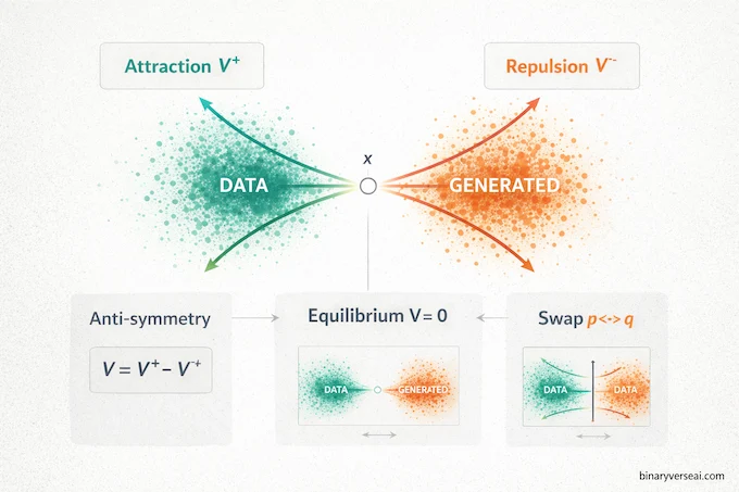
Here’s the key proposition: if the drifting field is anti-symmetric, swapping the data distribution and the generated distribution flips the sign of the drift. The paper states:
If q = p, then V(x) = 0 for all x.
This is the equilibrium guarantee. It’s not optional decoration.
Now the fun part: they do a destructive ablation where they intentionally break the balance between attraction and repulsion. It explodes. FID goes from 8.46 in the default anti-symmetric setting to 41, 46, 86, even 177 when you mess with the symmetry or remove repulsion.
That’s the practical meaning of anti-symmetry drifting models: not “math purity,” but “this is the difference between converging and faceplanting.”
5.1. The Intuition You Can Reuse
When p and q match, you want attraction and repulsion to cancel. Otherwise, even at the correct distribution you’d keep drifting, which is like a thermostat that keeps heating after it reaches the setpoint.
6. The Training Objective: Stop-Grad “Drifted Target” And Why It Works
Once you have a drift vector, the naive thing would be to differentiate through it. But V depends on the generated distribution, and “backprop through a distribution” is where many clean ideas go to die.
So the paper does something that feels very modern-deep-learning: create a frozen target using stop-gradient.
They define a fixed-point style update, then turn it into a loss that pulls the prediction toward x + V(x), with the “drifted” point treated as a constant for that iteration.
Crucially, they note that the value of this loss equals the expected squared norm of the drift, E[‖V‖²], but the optimization path avoids directly backpropagating through V.
If you’ve built systems like BYOL, SimSiam, or consistency-style training loops, this pattern feels familiar: make an update target that you don’t differentiate through, then chase it.
7. Designing V: Kernels, Soft Assignments, And The Temperature τ Headache
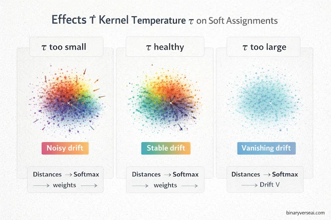
The kernel is where drift becomes geometry. They use:
k(x, y) = exp( − (1/τ) ‖x − y‖ )
with τ as a temperature.
Implementation detail that matters: they compute a normalized kernel using softmax with logits −(1/τ)‖x − y‖, taken over y.
Then they do something extra: an additional softmax normalization over x within the batch, which slightly improves performance while preserving anti-symmetry.
7.1. Rules Of Thumb For τ (From Pain, Not Poetry)
This is where people burn hours. Here’s a practical way to think about kernel temperature tau drifting models:
- Too small τ: the kernel becomes almost one-hot. Drift becomes noisy and brittle. You chase nearest neighbors like a dog seeing squirrels.
- Too large τ: the kernel goes flat. Everything looks equally far. Drift vanishes and training starves.
- Healthy τ: you get meaningful neighborhoods. Nearby points matter more, but not exclusively.
If your drift norms go to near zero early while samples still look awful, you probably have the “flat kernel” problem the authors mention, where all points are far and k(·,·) effectively vanishes.
8. Multi-Temperature Drifting: How They Stabilize Multi-Scale Structure
The paper includes a simple and very sane trick: compute drift at multiple temperatures and aggregate it. In their ablation default, τ values {0.02, 0.05, 0.2} together slightly beat the best single temperature and, more importantly, remove the need to retune τ across configs.
This is one of those “why didn’t I do that” ideas. Multi-temperature drift acts like multi-scale perception: small τ captures sharp local structure, larger τ captures broader semantic neighborhoods.
In practice, it’s also an engineering win. You spend less time doing the sacred ritual of hyperparameter roulette.
9. Feature Space Matters: Why A Strong Encoder Can Make Or Break The Method
The drift computation depends on distances. Distances in pixel space are famously stupid. Distances in a good feature space are often useful.
So the paper computes the drift loss in a feature space produced by an encoder ϕ. They emphasize two practical points:
- Feature encoding is training-time only, not used at inference.
- They compute losses across multiple scales and locations for richer gradients.
They also report something that’s refreshingly honest: they couldn’t make the method work on ImageNet without a feature encoder, likely because the kernel fails to describe similarity when everything is far apart.
If you want a single takeaway to tape above your monitor: your drift is only as good as your notion of “near.”
10. Drifting Models Vs Diffusion, Flow, Consistency: The Clean Comparison Readers Want
Let’s compress the comparison into one sentence:
Diffusion and flow matching do many small updates at inference, Drifting Models aim to do those updates during training, so inference becomes one jump.
10.1. What’s Similar
- All of these families are trying to match distributions, not labels.
- All of them benefit from strong architectures and guidance tricks.
- All of them hide a lot of magic inside “what is your training signal and where does it come from.”
10.2. What’s Actually Different
- No SDE/ODE solver at sampling time.
- The “trajectory” is the optimizer’s sequence of models and pushforward distributions.
- The training objective is literally about reducing drift norm, not denoising noise levels or matching vector fields.
Also, a practical note: many one-step methods in the literature are distilled from multi-step teachers. The paper stresses their best numbers come from native 1-NFE generation, trained from scratch.
That’s a big claim, and it’s why this direction feels like more than a speed hack.
11. Benchmarks That Matter: ImageNet 256×256 One-Step Results (And What’s Fair To Claim)
The headline is not subtle: state-of-the-art one-step generation on ImageNet 256×256, plus pixel-space results that punch hard.
Let’s anchor it with the system-level comparison tables.
11.1. What The Numbers Actually Say
In latent space, their larger model hits FID 1.54 at NFE 1.
In pixel space, their larger model hits FID 1.61 at NFE 1.
Here’s a condensed view:
| Setting | Method | NFE | FID (↓) | Notes |
|---|---|---|---|---|
| Latent (ImageNet 256×256) | Drifting Model, L/2 | 1 | 1.54 | Trained from scratch |
| Latent (ImageNet 256×256) | iMeanFlow-XL/2 | 1 | 1.72 | Single-step diffusion/flow family |
| Latent (ImageNet 256×256) | DiT-XL/2 | 250×2 | 2.27 | Multi-step baseline |
| Pixel (ImageNet 256×256) | Drifting Model, L/16 | 1 | 1.61 | Pixel-space one-step |
| Pixel (ImageNet 256×256) | PixelDiT/16 | 200×2 | 1.61 | Strong multi-step pixel model |
11.2. What’s Fair To Claim
- The method is genuinely competitive at ImageNet scale in a one-step regime.
- The training recipe leans on a strong feature encoder and careful kernel behavior, this is not “just plug and play.”
- “One-step” does not mean “no complexity,” it means the complexity moves into training dynamics and drift estimation.
Also, if you’re the type who wants a sanity check: the paper shows that breaking anti-symmetry catastrophically degrades FID. That’s a strong indicator the mechanism is doing real work, not just riding architecture luck.
12. Minimal Implementation Path: What To Code First, Common Bugs, And Sanity Checks
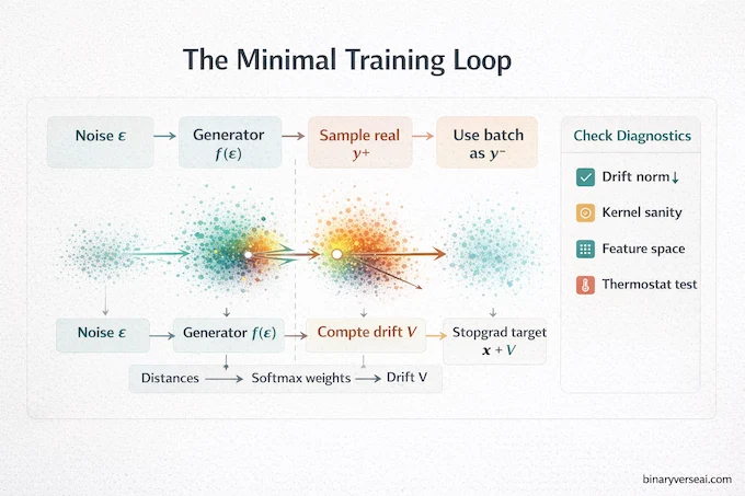
If you want to implement this without turning your life into an interpretive dance called “Why Is My Drift NaN,” here’s the shortest path.
12.1. The Minimum Loop
The paper’s Algorithm 1 is basically:
- Sample noise ε
- Generate x = f(ε)
- Sample positives y⁺ from data
- Use generated samples as negatives y⁻
- Compute V(x, y⁺, y⁻)
- Set target as stopgrad(x + V)
- Regress x toward target with MSE
That’s all you need to get a toy 2D case running.
12.2. The Debug Checklist That Pays Rent
A. Drift sanity
- Print mean ‖V‖. It should start nonzero and trend down over training. The paper explicitly links training progress to decreasing ‖V‖².
- Visualize a few drift vectors in a toy space. If attraction and repulsion look identical, you likely broke your normalization.
B. Kernel sanity
- Plot pairwise distances. If everything is far, your kernel goes flat and drift disappears.
- Try multi-temperature aggregation early. It’s a cheap stabilizer.
C. Feature space sanity
- If you’re in high dimensions, start with a decent encoder. The paper’s ImageNet results rely on feature-space drifting, and they note failure without it.
- Remember: the encoder is training-time only, so don’t optimize it for inference constraints.
D. Anti-symmetry sanity
- If you “improve” the method by weighting attraction more than repulsion, expect it to get worse. The destructive ablations are brutal.
12.3. A Small, Practical Repro Tip
Treat drift computation like a first-class module. Unit test it on small arrays. Verify:
- swapping positives and negatives flips the sign, at least approximately
- increasing τ smooths assignments
- setting positives equal to negatives drives drift toward zero
That last check is your “thermostat” test.
Closing: Why This Direction Feels Like A Big Deal
One-step generators have been a long-running dream because they promise the best of both worlds: diffusion-grade quality with the serving simplicity of a single forward pass. The reason it usually doesn’t work is also simple: distribution matching is hard, and iterative solvers are a crutch that helps.
Drifting Models is interesting because it doesn’t just try to crank the same handle faster. It reframes where the iteration lives. The drift field gives you an explicit mechanism, and anti-symmetry gives you an equilibrium story that holds up in practice.
If you build generative systems, this is worth more than a skim. Read Generative Modeling via Drifting, then try a toy implementation, then try swapping encoders and τ values until you can feel the kernel geometry in your bones.
If you want, paste your current training loop or kernel code and I’ll help you tighten it, add the right sanity checks, and get to a stable “it actually learns” baseline fast.
What Is Model Drifting?
In production ML, “model drift” means a deployed model degrades because the world and the data change. In Drifting Models, “drifting” is a generative training mechanism where samples move under a learned field so inference can be one-step.
What Is Meant By Drifting Here?
“Drifting” means you update a generated sample with a learned step like x ← x + V(x). The drifting field V is computed from real samples (pull) and generated samples (push) so the generator learns the whole refinement process during training.
3. What Is Model Drift In Machine Learning?
Model drift is when a model’s real-world accuracy drops over time because the input distribution, label relationship, or environment changes. It’s a monitoring and retraining problem, not a generative modeling method.
What Is LLM Model Drift?
LLM drift is the same idea applied to language models, user prompts change, tool outputs shift, policies evolve, or a product’s traffic mix changes, so behavior and quality move. That’s separate from Drifting Models, which is about one-step generative sampling.
5. What Is Model Drift Vs Data Drift?
Data drift is the input distribution changing. Model drift is the performance drop that follows, often caused by data drift or concept drift. Keep this distinction short so the page stays focused on generative intent.