
A beam splitter is simple enough to draw on a napkin. Proving the sharp entropy bound for everything that can enter its two ports took considerably more machinery. OpenAI’s September 24, 2026 manuscript presents an entropy photon number inequality proof for independent finite-energy bosonic inputs, allowing arbitrary entanglement among modes within either input.
The result bounds the retained output’s entropy-equivalent photon occupation by a weighted combination of the two input values. It resolves the conjecture in the manuscript’s finite-energy setting and yields exact thermal-channel entropy minima and a specific optical broadcast capacity region. These are mathematical results, rather than measured improvements to optical hardware. A public formalization discrepancy, explained below, also limits what can presently be called machine verified.
Table of Contents
1. What Is the Entropy Photon-Number Inequality, and What Did OpenAI Prove?
Guha, Erkmen, and Shapiro introduced the entropy photon-number conjecture in 2007. Its central comparison asks whether arbitrary independent quantum inputs produce at least as much entropy as appropriately matched thermal inputs. The roughly nineteen-year interval measures the problem’s history, not the duration of OpenAI’s computation.
| Question | Precise Scope |
|---|---|
| Inputs | Two independent systems, each with the same finite positive number of bosonic modes. |
| Energy | Each input has finite total mean photon number. |
| Correlations | Entanglement within either input is permitted. |
| Output | One retained port after passive beam-splitter mixing. |
| Status | Released proof manuscript; linked Lean comparator contains an unfinished proof. |
The research paper’s Theorem 1.1 is the central result. Optical communication consequences follow from it under additional channel assumptions. OpenAI’s mathematics release attributes the collection to an internal frontier model, without establishing this paper’s individual degree of human involvement.
2. The Original Problem: What Happens When Independent Quantum Light Inputs Mix?
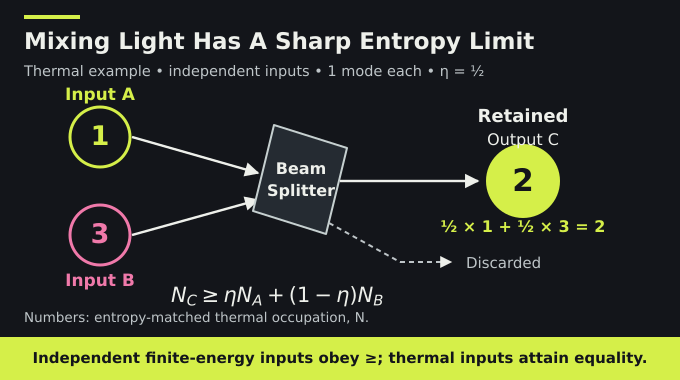
A bosonic mode is a quantum harmonic oscillator whose occupation can be zero, one, two, or arbitrarily many photons. For each mode index, a beam splitter mixes annihilation operators and . Its power transmissivity weights the first port:
The full optical transformation is unitary and preserves combined photon number. The theorem concerns only one output, obtained by tracing out the other. That distinction matters: a subsystem’s entropy can change even when the joint system undergoes reversible evolution. Our 2D area-law explainer develops the related idea of reduced-state entropy.
Independence means the joint input is . It does not require separate modes inside either port to be independent. There is no assumption that the two physical outputs are independent either.
3. Understanding the Entropy Photon Number Inequality Formula
Von Neumann entropy is . Natural logarithms make its units nats. A thermal mode with mean occupation has entropy:
Use the continuous convention . The function increases from zero without bound, so it has an inverse. For an -mode state, define the effective entropy photon number:
This is the occupation per mode of an identical product thermal reference with matching total entropy. It need not equal the state’s actual mean occupation. Theorem 1.1 assumes finite mean photon number at each input and states:
For one thermal mode at each port with occupations one and three, balanced mixing produces occupation two. The respective entropies are approximately 1.386294, 2.249341, and 1.909543 nats. Applying the inverse thermal-entropy function gives exactly one, three, and two, attaining equality. This checks the formula without pretending to test arbitrary quantum inputs.
Notice that the output entropy lies below the hotter input’s entropy. The theorem does not say that mixing makes the retained light more disordered than either source individually. It identifies the sharp lower comparison after translating entropy into thermal occupation. Photon number here is an entropy scale, rather than a count obtained from a detector.
4. Why Earlier Quantum Entropy Power Inequalities Were Not Enough
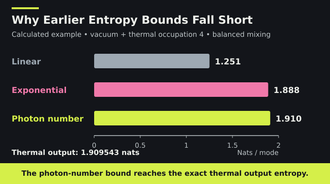
The linear bound puts output entropy above the transmissivity-weighted input entropies. The stronger quantum entropy power inequality instead compares their exponentials:
If input entropies match, the linear bound already gives the photon-number result. Unequal levels expose the difference. Consider vacuum and a thermal mode of occupation four at balanced mixing. The exact output is thermal with occupation two.
The photon-number inequality was previously known for independent Gaussian inputs, including internal Gaussian correlations. One-mode constrained entropy minima and additional multimode cases were also established. The new manuscript addresses two freely varying non-Gaussian inputs and unrestricted internal entanglement, rather than replacing those earlier results.
5. The Mathematical Foundation: Thermal States, Energy Bounds, and Compactness
Fock space has number-basis vectors labeling each mode’s occupation. The total number operator is unbounded. Finite mean energy therefore controls an infinite-dimensional state space, rather than turning it into a finite matrix problem. The continuum issue has a different form in our electronic-structure hardness explainer.
For positive occupation , the reference thermal state is proportional to , where . It has total occupation and entropy . Relative entropy measures departure from this reference and is nonnegative.
In particular, equals minus the state’s entropy, plus , plus . This identity links entropy and energy. Because maximal entropy grows only logarithmically with energy at fixed mode count, a positive linear energy penalty can dominate the negative entropy terms in the later optimization.
Lemma 2.2 supplies compactness in trace norm under a common finite energy bound, together with entropy continuity and the upper bound when total occupation is at most . Number cutoffs control the high-energy tail. These facts make limiting arguments possible without assuming energy itself converges. Thermal references here serve a different purpose from macroscopic ordering in our Bose–Einstein condensation explainer.
6. The New Mathematical Ingredient: Four-Weight Interpolation
Theorem 3.1 concerns positive diagonal quadratic forms: weighted sums of squared coordinates. A comparison says one source form dominates a weighted sum of transformed target forms. The same comparison is assumed for four weights:
Here , the parameters are real, and . Source tests use finitely many parameter values and are stable under functions of those parameters. No compatibility between the linear maps and diagonal multipliers is assumed. The theorem transfers comparison to:
The proof combines positive sums, limits, logarithmic means, and parallel sums. A Stieltjes representation expresses a needed derivative through positive resolvent kernels, enabling another admissible weight. A final quadratic minimization produces exactly the displayed ratio. Multiplying two valid weights would not justify that step. This construction supplies the particular thermal-relaxation metric the contradiction argument needs.
7. How OpenAI Constructs a Regularized Counterexample
Assume a strict violation exists. Finite-number truncations preserve a violation, allowing a finite-support witness. Fix positive thermal reference occupations equal or close to the witness’s entropy photon numbers. These reference parameters remain fixed during optimization.
| Device | Role In The Argument |
|---|---|
| Auxiliary thermal port | Creates slack for the metric comparisons. |
| Thermal output replacement | Bounds the output’s negative logarithm. |
| Relative-entropy penalty | Controls energy and supplies a strict final margin. |
| Fourth-moment penalty | Justifies calculations with unbounded operators. |
The objective combines output entropy deviation, weighted input entropy deviations, and these positive penalties. Parameters are chosen so its minimum remains uniformly negative. Energy coercivity prevents minimizing sequences from escaping to arbitrarily large occupation.
Each entropy deviation is measured relative to its fixed thermal reference and divided by the corresponding . This converts the deviations to the local photon-number scale, since . Output replacement means a convex mixture with a thermal state, distinct from the additional thermal input port. Confusing those operations obscures why their regularizing effects differ.
At a minimum, varying one input identifies a faithful Gibbs state. Faithful means no zero eigenvalues, making logarithms manageable. The regularized inputs acquire finite seventh moments, stronger control than initially imposed. Crucially, only the fourth-moment penalty coefficient tends to zero at the end. Sending every regularization parameter to zero would describe a different argument.
8. Entropy-Hessian Estimates and the Thermal Relaxation Metric
Stationarity gives identities for each input’s negative logarithm in terms of an output-observable slice, an energy term, and the moment penalty. Second-order relative-entropy comparisons then yield component contractions at those minimizing states. They are not asserted as universal inequalities for arbitrary channel inputs.
The relevant observable metric weights matrix entries using the logarithmic mean , continuously extended at equality. Ratios of state eigenvalues define modular frequencies. Two variance comparisons from independent ports and two constant-weight comparisons provide the four interpolation hypotheses.
Their combination controls centered thermal-balance defect functionals. These test how creation and annihilation expectations depart from the reference thermal balance after subtracting the mean field. Centering removes coherent displacement, so a displaced thermal state also has zero centered defect. The proof must therefore control the input means separately. This is a useful warning: a quantity can certify one structural feature while leaving another undetermined. Our Heisenberg ferromagnet explainer similarly distinguishes thermal structure from a chosen order parameter.
9. The Decisive Step: Stationarity, Cancellation, and the Thermal Limit
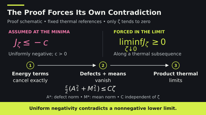
Section 6 pairs the Gibbs identities with thermal-relaxation generators. Entropy production separates into a squared defect norm and a centered-energy correction. Combining input and output identities cancels those energy corrections exactly. The resulting estimate is:
Here is fixed, sums weighted input defect norms, sums weighted squared means, and is independent of . Both defects and means therefore vanish as that coefficient decreases.
Uniform energy bounds produce trace-norm limits. Testing against fixed finite number-basis matrices gives the balance relation . Its entries force off-diagonal terms to vanish and diagonal probabilities to have geometric ratios. Normalization identifies each limit as the reference product thermal state, eliminating internal correlations as well.
The diagonal ratio is whenever one occupation increases by one. Repeating that relation in every mode fixes the whole joint probability distribution. Thus thermal structure is deduced from operator identities, rather than inserted as an optimizer assumption.
Entropy continuity now sends the objective’s entropy portion to zero. The remaining penalties are nonnegative, contradicting the uniformly negative minimum. Neither penalty must itself converge to zero. The proof also avoids assuming differentiability of entropy along an unbounded evolution.
10. What the Proof Establishes for Minimum Output Entropy
A thermal attenuator mixes an input with an independent thermal environment of occupation . For identical channel parameters across all modes, fix input entropy . Corollary 1.2 gives:
Applying the inequality to the input and environment proves the lower bound. A product thermal input of occupation attains it because thermal occupations mix linearly. Arbitrary internal entanglement was permitted in the optimization, so entangled inputs cannot improve this constrained minimum.
Attainment does not prove uniqueness. The corollary concerns identical passive thermal attenuators, rather than mode-dependent attenuation, amplifiers, or additive-noise channels. Nor does an exact optimum provide a faster simulation algorithm, a distinction also relevant to our QAOA theorem explainer.
11. Optical Communication Capacity: Exact Results and Their Limits
Corollary 7.1 treats two receivers with transmissivities and . Auxiliary ports are vacuum. With codebook-and-use averaged photon occupation , the capacity region is the closed convex hull of nonnegative rate pairs satisfying, for some :
Rates are nats per use. The vacuum specialization supplies the converse entropy bound; coherent-state superposition coding supplies achievability. Messages are independent, decoding errors vanish on average, receivers decode collectively but separately, and neither feedback nor cooperation is allowed. This is an asymptotic coding theorem, without a demonstrated receiver implementation.
The parameter controls the tradeoff. Increasing it raises the stronger receiver’s private-message rate while reducing the weaker receiver’s available rate. Coherent-state superposition combines independently Gaussian-distributed amplitude layers. In the converse, degradation means the weaker marginal can be generated by further attenuation of the stronger one, not that the receivers’ outputs are independent.
The Lean scope note describes the central inequality and excludes both corollaries. However, its linked comparator theorem ends in sorry. That placeholder does not constitute a completed proof. This article explains the manuscript without claiming independent Lean verification or peer-review acceptance. Our Lean formalization explainer provides further context.
The entropy photon number inequality offers a sharp thermal benchmark for quantum optical information. Follow Binary Verse AI’s research explainers and companion videos to work through the mechanisms, assumptions, and verification evidence behind results like this one.
Is entropy photon number the same as entropy per photon?
No. Entropy photon number is the mean occupation per mode of an identical product thermal reference with the same total entropy as the state. It is not a universal amount of entropy carried by each photon.
Does mixing light through a beam splitter always increase entropy?
Not in the sense of exceeding both input entropies. The theorem lower-bounds the retained output’s effective entropy photon number by the transmissivity-weighted input values. This need not put the output entropy above the larger input entropy.
Does the inequality remain valid for entangled quantum states?
The manuscript allows arbitrary entanglement among modes within either input. The two input systems must nevertheless be independent, with joint state the tensor product of the two input states, and each must have finite mean energy.
Why couldn’t earlier quantum entropy power inequalities resolve the conjecture?
Earlier inequalities gave weaker entropy lower bounds. For unequal input entropy levels, they did not reproduce the exact thermal-state comparison required by the photon-number conjecture. Equal entropy levels were already covered by the linear entropy bound.
When does the entropy photon-number inequality become an equality?
Independent product thermal inputs attain equality when all modes within each port share a common mean occupation, including when the two ports have different occupations. The theorem asserts attainment, rather than a classification of all equality cases.
Does OpenAI’s proof determine the capacity of every optical communication channel?
No. The manuscript determines the capacity region for a specified degraded two-receiver pure-loss bosonic broadcast channel with independent classical messages, a mean photon constraint, separate collective decoding, and no feedback or receiver cooperation. It does not determine capacities for arbitrary amplifiers, noisy channels, or networks.